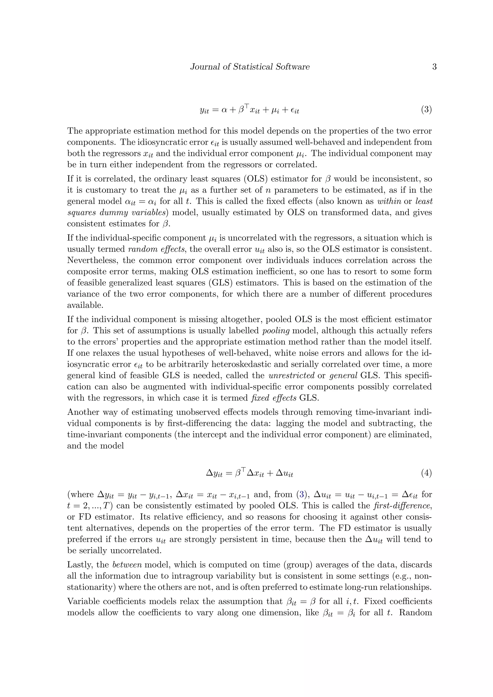
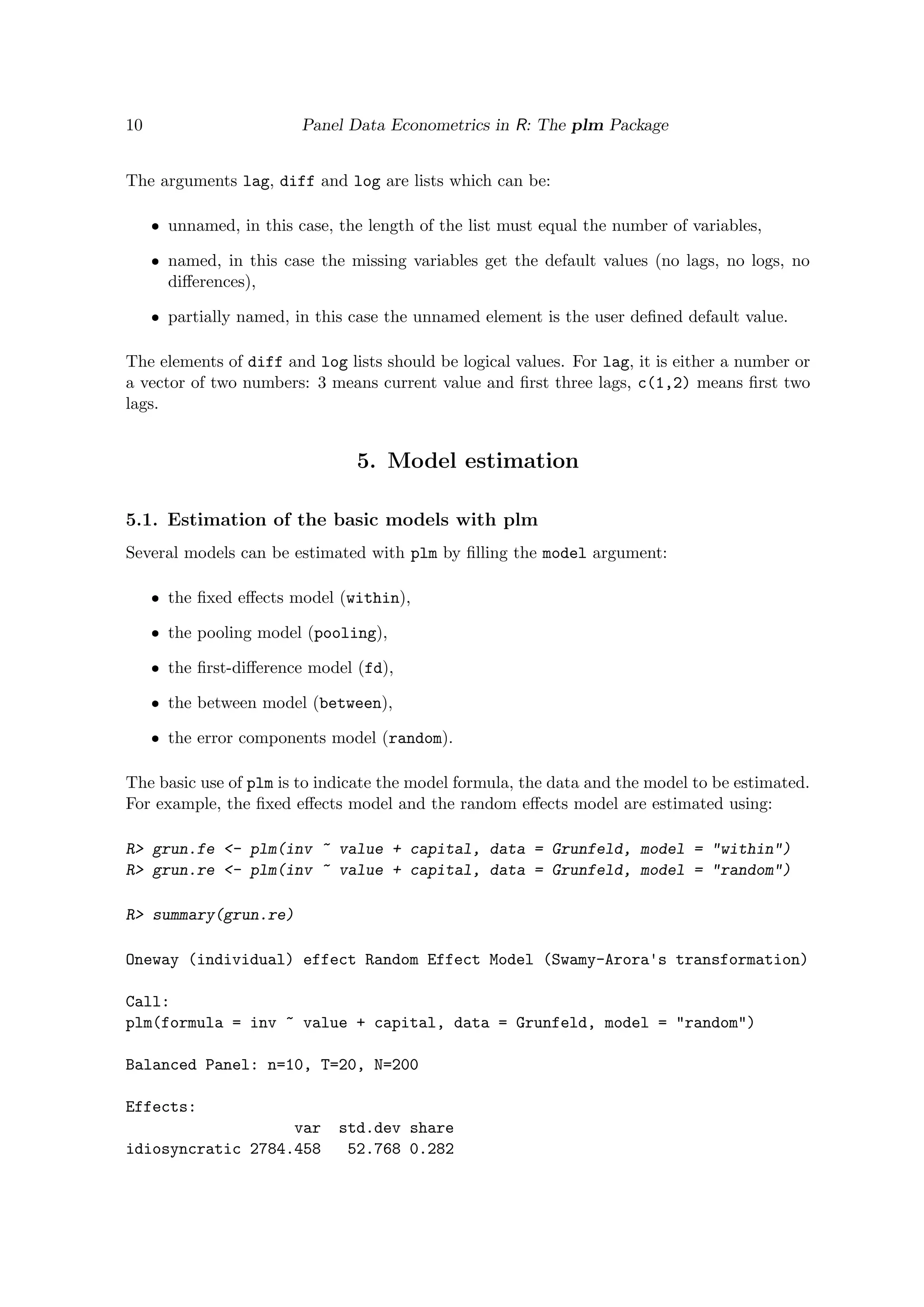
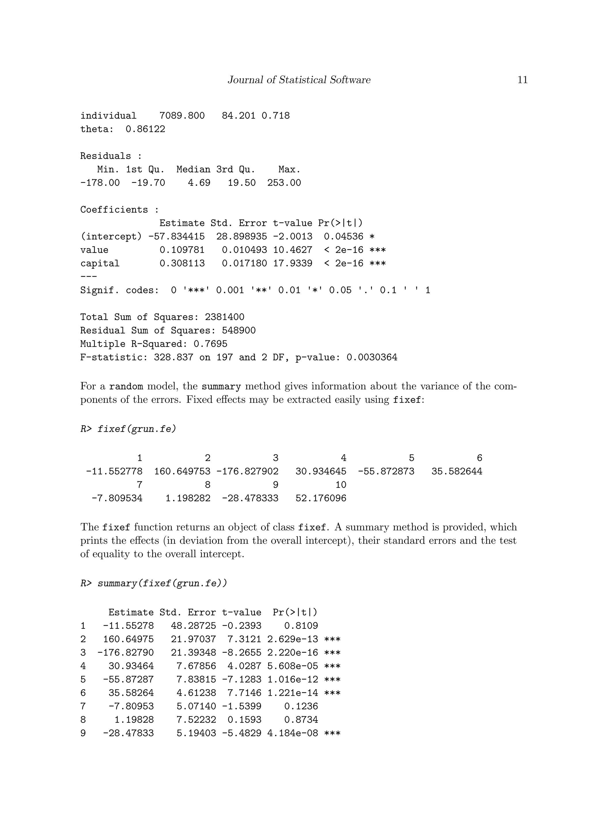
This document introduces the plm package for panel data econometrics in R. It discusses panel data models and estimation approaches, describes the software approach and functions in plm, and compares plm to other R packages for longitudinal data analysis. Key features of plm include functions for estimating linear panel models with fixed effects, random effects, and GMM, as well as data management and diagnostic testing capabilities for panel data. The package aims to make panel data analysis intuitive and straightforward for econometricians in R.


![6 Panel Data Econometrics in R: The plm Package
inexpensive. Therefore most examples in the following are based on formula methods, which
are perhaps the cleanest for illustrative purposes.
3.3. Computational approach to estimation
The feasible GLS methods needed for efficient estimation of unobserved effects models have
a simple closed-form solution: once the variance components have been estimated and hence
the covariance matrix of errors ˆV , model parameters can be estimated as
ˆβ = (X ˆV −1
X)−1
(X ˆV −1
y) (5)
Nevertheless, in practice plain computation of ˆβ has long been an intractable problem even
for moderate-sized datasets because of the need to invert the N × N ˆV matrix. With the
advances in computer power, this is no more so, and it is possible to program the “naive”
estimator (5) in R with standard matrix algebra operators and have it working seamlessly for
the standard “guinea pigs”, e.g., the Grunfeld data. Estimation with a couple of thousands
of data points also becomes feasible on a modern machine, although excruciatingly slow and
definitely not suitable for everyday econometric practice. Memory limits would also be very
near because of the storage needs related to the huge ˆV matrix. An established solution
exists for the random effects model which reduces the problem to an ordinary least squares
computation.
The (quasi-)demeaning framework
The estimation methods for the basic models in panel data econometrics, the pooled OLS,
random effects and fixed effects (or within) models, can all be described inside the OLS
estimation framework. In fact, while pooled OLS simply pools data, the standard way of
estimating fixed effects models with, say, group (time) effects entails transforming the data
by subtracting the average over time (group) to every variable, which is usually termed time-
demeaning. In the random effects case, the various feasible GLS estimators which have been
put forth to tackle the issue of serial correlation induced by the group-invariant random effect
have been proven to be equivalent (as far as estimation of βs is concerned) to OLS on partially
demeaned data, where partial demeaning is defined as:
yit − θ¯yi = (Xit − θ ¯Xi)β + (uit − θ¯ui) (6)
where θ = 1−[σ2
u/(σ2
u +Tσ2
e )]1/2, ¯y and ¯X denote time means of y and X, and the disturbance
vit − θ¯vi is homoskedastic and serially uncorrelated. Thus the feasible RE estimate for β may
be obtained estimating ˆθ and running an OLS regression on the transformed data with lm().
The other estimators can be computed as special cases: for θ = 1 one gets the fixed effects
estimator, for θ = 0 the pooled OLS one.
Moreover, instrumental variable estimators of all these models may also be obtained using
several calls to lm().
For this reason the three above estimators have been grouped inside the same function.
On the output side, a number of diagnostics and a very general coefficients’ covariance matrix
estimator also benefits from this framework, as they can be readily calculated applying the](https://image.slidesharecdn.com/glm-150815235210-lva1-app6892/75/Glm-6-2048.jpg)
![Journal of Statistical Software 7
standard OLS formulas to the demeaned data, which are contained inside plm objects. This
will be the subject of Section 3.4.
The object oriented approach to general GLS computations
The covariance matrix of errors in general GLS models is too generic to fit the quasi-demeaning
framework, so this method calls for a full-blown application of GLS as in (5). On the other
hand, this estimator relies heavily on n-asymptotics, making it theoretically most suitable
for situations which forbid it computationally: e.g., “short” micropanels with thousands of
individuals observed over few time periods.
R has general facilities for fast matrix computation based on object orientation: particular
types of matrices (symmetric, sparse, dense etc.) are assigned the relevant class and the
additional information on structure is used in the computations, sometimes with dramatic
effects on performance (see Bates 2004) and packages Matrix (see Bates and Maechler 2007)
and SparseM (see Koenker and Ng 2007). Some optimized linear algebra routines are available
in the R package kinship (see Atkinson and Therneau 2007) which exploit the particular block-
diagonal and symmetric structure of ˆV making it possible to implement a fast and reliable
full-matrix solution to problems of any practically relevant size.
The ˆV matrix is constructed as an object of class bdsmatrix. The peculiar properties of this
matrix class are used for efficiently storing the object in memory and then by ad-hoc versions
of the solve and crossprod methods, dramatically reducing computing times and memory
usage. The resulting matrix is then used “the naive way” as in (5) to compute ˆβ, resulting in
speed comparable to that of the demeaning solution.
3.4. Inference in the panel model
General frameworks for restrictions and linear hypotheses testing are available in the R en-
vironment4. These are based on the Wald test, constructed as ˆβ ˆV −1 ˆβ, where ˆβ and ˆV are
consistent estimates of β and V (β), The Wald test may be used for zero-restriction (i.e., signifi-
cance) testing and, more generally, for linear hypotheses in the form (R ˆβ−r) [R ˆV R ]−1(R ˆβ−
r)5. To be applicable, the test functions require extractor methods for coefficients’ and covari-
ance matrix estimates to be defined for the model object to be tested. Model objects in plm
all have coef() and vcov() methods and are therefore compatible with the above functions.
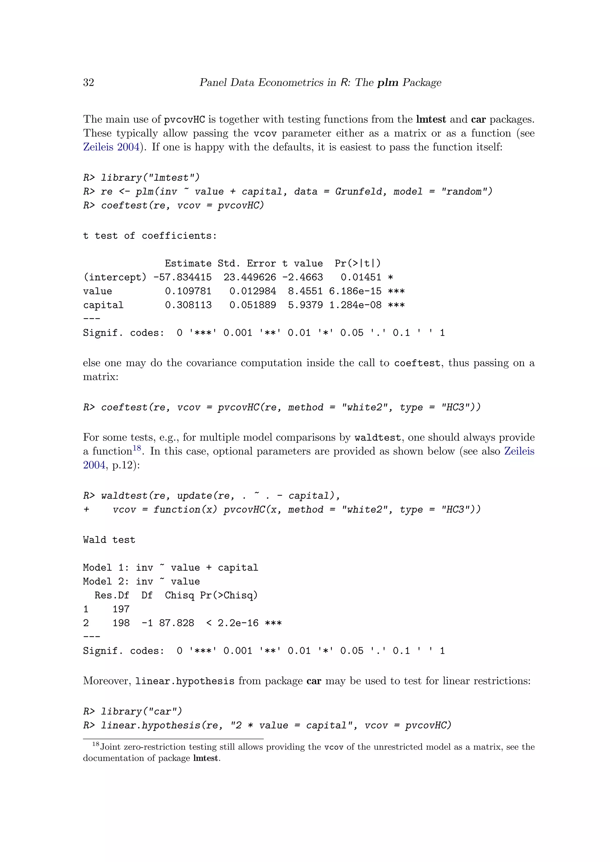
In the same framework, robust inference is accomplished substituting (“plugging in”) a robust
estimate of the coefficient covariance matrix into the Wald statistic formula. In the panel
context, the estimator of choice is the White system estimator. This called for a flexible
method for computing robust coefficient covariance matrices `a la White for plm objects.
A general White system estimator for panel data is:
ˆVR(β) = (X X)−1
n
i=1
Xi EiXi(X X)−1
(7)
where Ei is a function of the residuals ˆeit, t = 1, . . . T chosen according to the relevant
heteroskedasticity and correlation structure. Moreover, it turns out that the White covariance
4
See packages lmtest (Zeileis and Hothorn 2002) and car (Fox 2007).
5
Moreover, coeftest() provides a compact way of looking at coefficient estimates and significance diag-
nostics.](https://image.slidesharecdn.com/glm-150815235210-lva1-app6892/75/Glm-7-2048.jpg)


![Journal of Statistical Software 23
For these reasons, the subjects of testing for individual error components and for serially
correlated idiosyncratic errors are closely related. In particular, simple (marginal) tests for one
direction of departure from the hypothesis of spherical errors usually have power against the
other one: in case it is present, they are substantially biased towards rejection. Joint tests are
correctly sized and have power against both directions, but usually do not give any information
about which one actually caused rejection. Conditional tests for serial correlation that take
into account the error components are correctly sized under presence of both departures from
sphericity and have power only against the alternative of interest. While most powerful if
correctly specified, the latter, based on the likelihood framework, are crucially dependent on
normality and homoskedasticity of the errors.
In plm we provide a number of joint, marginal and conditional ML-based tests, plus some
semiparametric alternatives which are robust versus heteroskedasticity and free from distri-
butional assumptions.
Unobserved effects test
The unobserved effects test `a la Wooldridge (see Wooldridge 2002, 10.4.4), is a semiparametric
test for the null hypothesis that σ2
µ = 0, i.e., that there are no unobserved effects in the
residuals. Given that under the null the covariance matrix of the residuals for each individual
is diagonal, the test statistic is based on the average of elements in the upper (or lower)
triangle of its estimate, diagonal excluded: n−1/2 n
i=1
T−1
t=1
T
s=t+1 ˆuit ˆuis (where ˆu are the
pooled OLS residuals), which must be “statistically close” to zero under the null, scaled by
its standard deviation:
W =
n
i=1
T−1
t=1
T
s=t+1 ˆuit ˆuis
[ n
i=1( T−1
t=1
T
s=t+1 ˆuit ˆuis)2]1/2
This test is (n-) asymptotically distributed as a standard Normal regardless of the distribution
of the errors. It does also not rely on homoskedasticity.
It has power both against the standard random effects specification, where the unobserved
effects are constant within every group, as well as against any kind of serial correlation. As
such, it “nests” both random effects and serial correlation tests, trading some power against
more specific alternatives in exchange for robustness.
While not rejecting the null favours the use of pooled OLS, rejection may follow from serial
correlation of different kinds, and in particular, quoting Wooldridge (2002), “should not be
interpreted as implying that the random effects error structure must be true”.
Below, the test is applied to the data and model in Munnell (1990):
R> pwtest(log(gsp) ~ log(pcap) + log(pc) + log(emp) + unemp, data = Produc)
Wooldridge's test for unobserved individual effects
data: formula
z = 3.9383, p-value = 8.207e-05
alternative hypothesis: unobserved effect
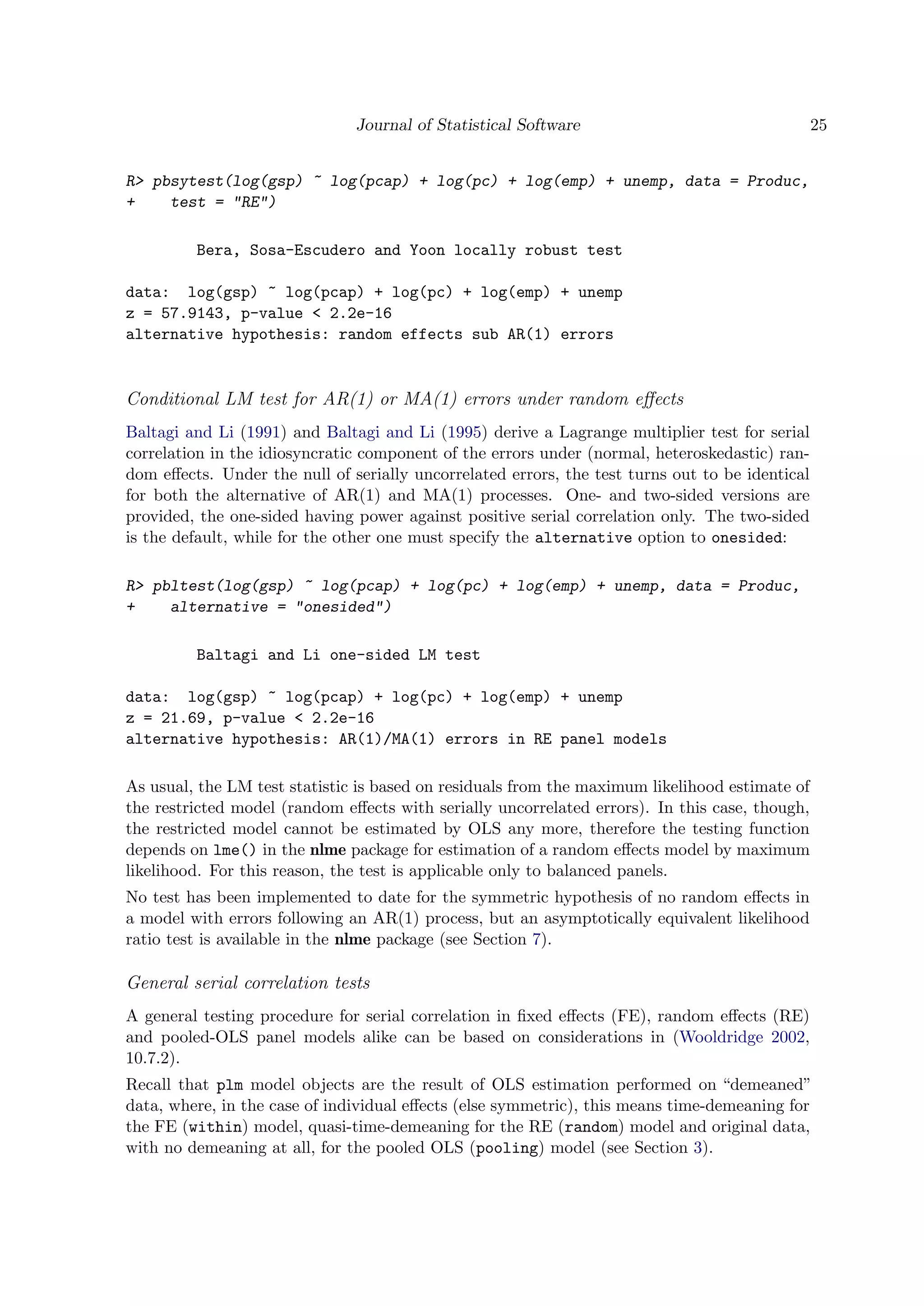
Locally robust tests for serial correlation or random effects
The presence of random effects may affect tests for residual serial correlation, and the opposite.](https://image.slidesharecdn.com/glm-150815235210-lva1-app6892/75/Glm-23-2048.jpg)

![26 Panel Data Econometrics in R: The plm Package
For the random effects model, Wooldridge (2002) observes that under the null of homoskedas-
ticity and no serial correlation in the idiosyncratic errors, the residuals from the quasi-
demeaned regression must be spherical as well. Else, as the individual effects are wiped
out in the demeaning, any remaining serial correlation must be due to the idiosyncratic com-
ponent. Hence, a simple way of testing for serial correlation is to apply a standard serial
correlation test to the quasi-demeaned model. The same applies in a pooled model, w.r.t. the
original data.
The FE case needs some qualification. It is well-known that if the original model’s errors
are uncorrelated then FE residuals are negatively serially correlated, with cor(ˆuit, ˆuis) =
−1/(T − 1) for each t, s (see Wooldridge 2002, 10.5.4). This correlation clearly dies out as T
increases, so this kind of AR test is applicable to within model objects only for T “sufficiently
large”11. On the converse, in short panels the test gets severely biased towards rejection (or,
as the induced correlation is negative, towards acceptance in the case of the one-sided DW
test with alternative = "greater"). See below for a serial correlation test applicable to
“short” FE panel models.
plm objects retain the “demeaned” data, so the procedure is straightforward for them. The
wrapper functions pbgtest and pdwtest re-estimate the relevant quasi-demeaned model by
OLS and apply, respectively, standard Breusch-Godfrey and Durbin-Watson tests from pack-
age lmtest:
R> grun.fe <- plm(inv ~ value + capital, data = Grunfeld, model = "within")
R> pbgtest(grun.fe, order = 2)
Breusch-Godfrey/Wooldridge test for serial correlation in
panel models
data: inv ~ value + capital
chisq = 42.5867, df = 2, p-value = 5.655e-10
alternative hypothesis: serial correlation in idiosyncratic errors
The tests share the features of their OLS counterparts, in particular the pbgtest allows
testing for higher-order serial correlation, which might turn useful, e.g., on quarterly data.
Analogously, from the point of view of software, as the functions are simple wrappers towards
bgtest and dwtest, all arguments from the latter two apply and may be passed on through
the ‘. . . ’ operator.
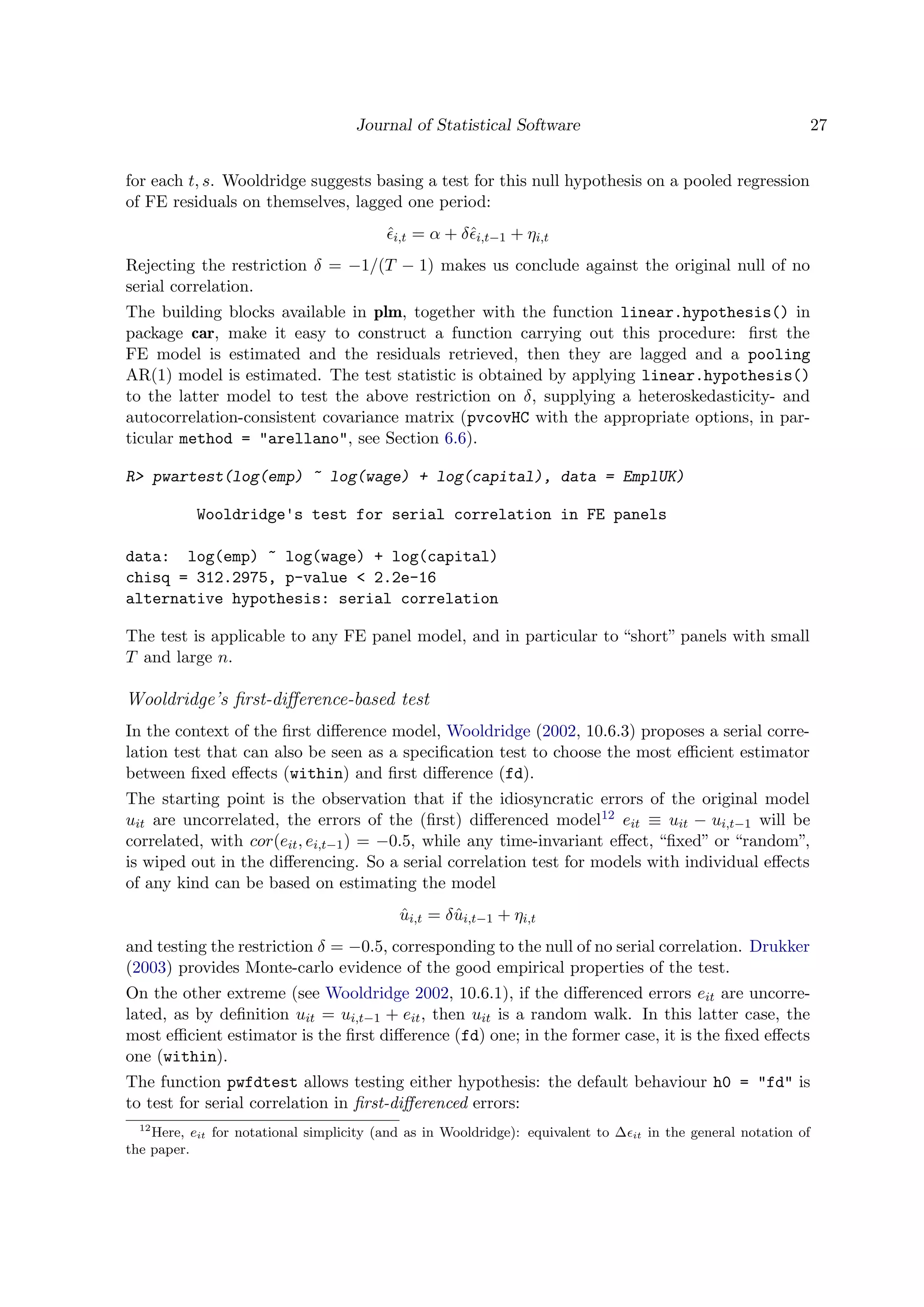
Wooldridge’s test for serial correlation in “short” FE panels
For the reasons reported above, under the null of no serial correlation in the errors, the
residuals of a FE model must be negatively serially correlated, with cor(ˆit, ˆis) = −1/(T −1)
11
Baltagi and Li derive a basically analogous T-asymptotic test for first-order serial correlation in a FE
panel model as a Breusch-Godfrey LM test on within residuals (see Baltagi and Li 1995, Paragraph 2.3 and
Formula 12). They also observe that the test on within residuals can be used for testing on the RE model,
as “the within transformation [time-demeaning, in our terminology] wipes out the individual effects, whether
fixed or random”. Generalizing the Durbin-Watson test to FE models by applying it to fixed effects residuals
is documented in Bhargava, Franzini, and Narendranathan (1982).](https://image.slidesharecdn.com/glm-150815235210-lva1-app6892/75/Glm-26-2048.jpg)
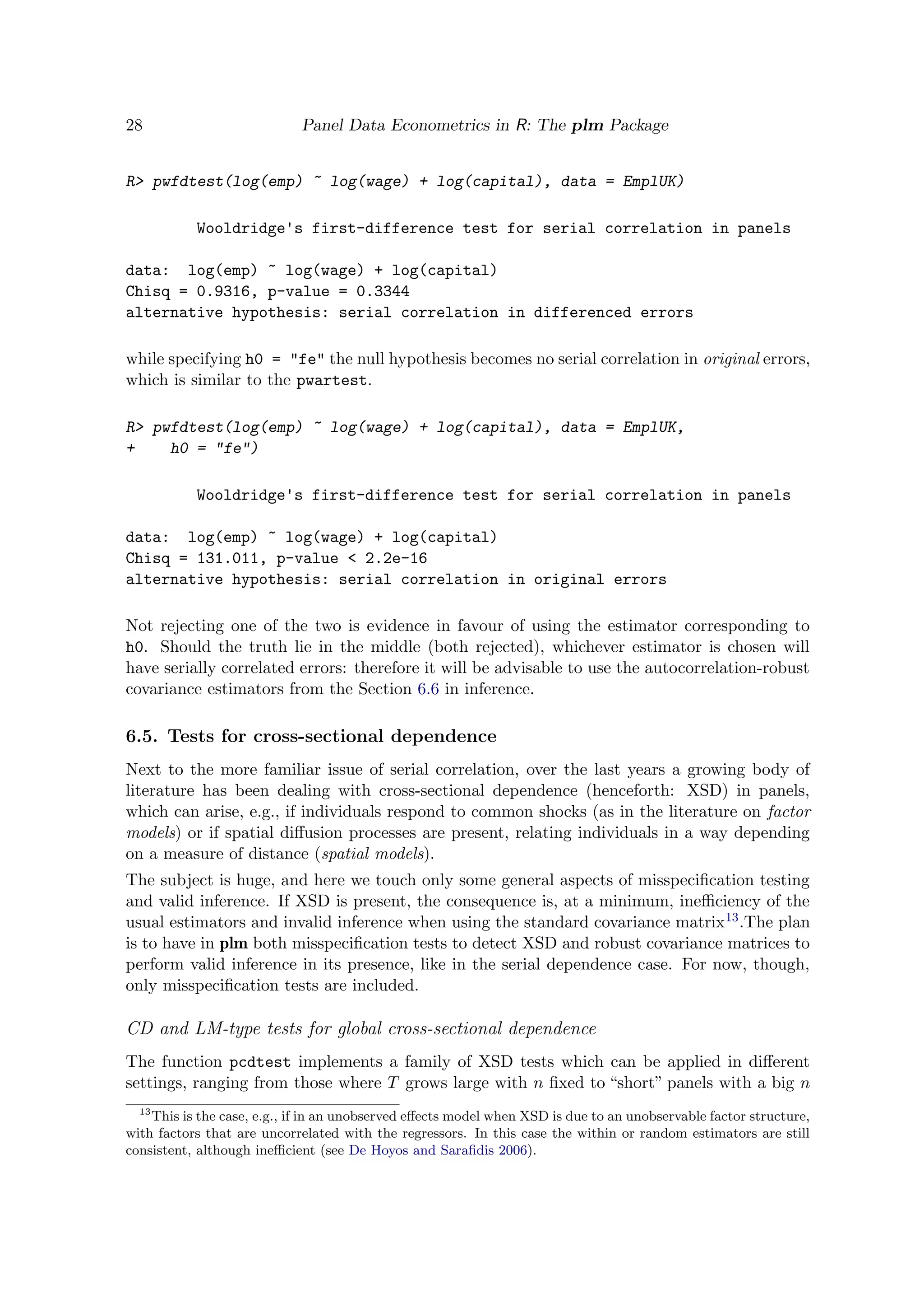

![30 Panel Data Econometrics in R: The plm Package
If a different model specification (within, random, ...) is assumed consistent, one can resort
to its residuals for testing14 by specifying the relevant model type. The main argument of this
function may be either a model of class panelmodel or a formula and a data.frame; in the
second case, unless model is set to NULL, all usual parameters relative to the estimation of a
plm model may be passed on. The test is compatible with any consistent panelmodel for the
data at hand, with any specification of effect. E.g., specifying effect = "time" or effect
= "twoways" allows to test for residual cross-sectional dependence after the introduction of
time fixed effects to account for common shocks.
R> pcdtest(inv ~ value + capital, data = Grunfeld, model = "within")
Pesaran CD test for cross-sectional dependence in panels
data: formula
z = 4.6612, p-value = 3.144e-06
alternative hypothesis: cross-sectional dependence
If the time dimension is insufficient and model=NULL, the function defaults to estimation of a
within model and issues a warning.
CD(p) test for local cross-sectional dependence
A local variant of the CD test, called CD(p) test (Pesaran 2004), takes into account an
appropriate subset of neighbouring cross-sectional units to check the null of no XSD against
the alternative of local XSD, i.e., dependence between neighbours only. To do so, the pairs
of neighbouring units are selected by means of a binary proximity matrix like those used in
spatial models. In the original paper, a regular ordering of observations is assumed, so that
the m-th cross-sectional observation is a neighbour to the (m − 1)-th and to the (m + 1)-th.
Extending the CD(p) test to irregular lattices, we employ the binary proximity matrix as a
selector for discarding the correlation coefficients relative to pairs of observations that are not
neighbours in computing the CD statistic. The test is then defined as
CD =
1
n−1
i=1
n
j=i+1 w(p)ij
n−1
i=1
n
j=i+1
[w(p)]ij Tij ˆρij
where [w(p)]ij is the (i, j)-th element of the p-th order proximity matrix, so that if h, k are
not neighbours, [w(p)]hk = 0 and ˆρhk gets “killed”; this is easily seen to reduce to formula
(14) in Pesaran (Pesaran 2004) for the special case considered in that paper. The same can
be applied to the LM and SCLM tests.
Therefore, the local version of either test can be computed supplying an n × n matrix (of any
kind coercible to logical), providing information on whether any pair of observations are
neighbours or not, to the w argument. If w is supplied, only neighbouring pairs will be used in
computing the test; else, w will default to NULL and all observations will be used. The matrix
14
This is also the only solution when the time dimension’s length is insufficient for estimating the heteroge-
neous model.](https://image.slidesharecdn.com/glm-150815235210-lva1-app6892/75/Glm-30-2048.jpg)


![Journal of Statistical Software 37
is done by creating an lmList object, so that the two models below are equivalent (output
suppressed):
R> vcmf <- pvcm(inv ~ value + capital, data = Grunfeld, model = "within",
+ effect = "time")
R> vcmfML <- lmList(inv ~ value + capital | year, data = Grunfeld)
Unrestricted FGLS
The general, or unrestricted, feasible GLS, pggls in the plm nomenclature, is equivalent to
a model with no random effects regressors (biq = 0 ∀i, q) and an error covariance structure
which is unrestricted within groups apart from the usual requirements. The function for
estimating such models with correlation in the errors but no random effects is gls().
This very general serial correlation and heteroskedasticity structure is not estimable for the
original Grunfeld data, which have more time periods than firms, therefore we restrict them
to firms 4 to 6.
R> sGrunfeld <- Grunfeld[Grunfeld$firm %in% 4:6, ]
R> ggls <- pggls(inv ~ value + capital, data = sGrunfeld, model = "random")
R> gglsML <- gls(inv ~ value + capital, data = sGrunfeld,
+ correlation = corSymm(form = ~ 1 | year))
R> coef(ggls)
(intercept) value capital
1.19679342 0.10555908 0.06600166
R> summary(gglsML)$coef
(Intercept) value capital
-2.4156266 0.1163550 0.0735837
The within case is analogous, with the regressors’ set augmented by n − 1 group dummies.
7.4. Some useful “econometric” models in nlme
Finally, amongst the many possible specifications estimable with nlme, we report a couple
cases that might be especially interesting to applied econometricians.
AR(1) pooling or random effects panel
Linear models with groupwise structures of time-dependence24 may be fitted by gls(), spec-
ifying the correlation structure in the correlation option:
R> lmAR1ML <- gls(inv ~ value + capital, data = Grunfeld,
+ correlation = corAR1(0, form = ~ year | firm))
24
Take heed that here, in contrast to the usual meaning of serial correlation in time series, we always speak
of serial correlation between the errors of each group.](https://image.slidesharecdn.com/glm-150815235210-lva1-app6892/75/Glm-37-2048.jpg)