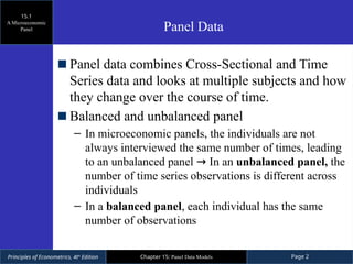
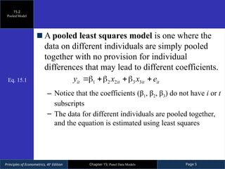
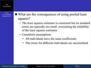
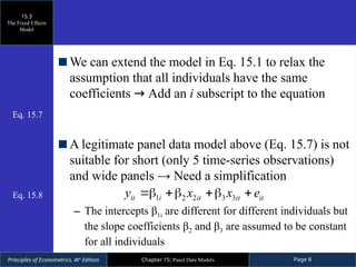
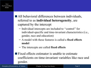
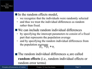
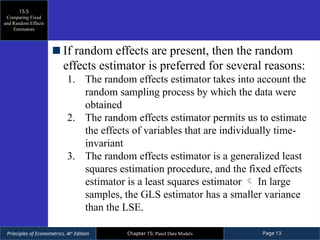
Principles of Econometrics, 4th
Edition Page 1
Chapter 15: Panel Data Models
Chapter 4
Panel Data Models
Principles of Econometrics, 4th
Edition Page 2
Chapter 15: Panel Data Models
Panel data combines Cross-Sectional and Time
Series data and looks at multiple subjects and how
they change over the course of time.
Balanced and unbalanced panel
– In microeconomic panels, the individuals are not
always interviewed the same number of times, leading
to an unbalanced panel → In an unbalanced panel, the
number of time series observations is different across
individuals
– In a balanced panel, each individual has the same
number of observations
15.1
A Microeconomic
Panel Panel Data
Principles of Econometrics, 4th
Edition Page 3
Chapter 15: Panel Data Models
15.1
A Microeconomic
Panel
Table 15.1 Representative Observations from NLS
(National Longitudinal Surveys) Panel Data
Principles of Econometrics, 4th
Edition Page 4
Chapter 15: Panel Data Models
15.2
A Microeconomic Panel: Pooled
Least Squares Estimates
Principles of Econometrics, 4th
Edition Page 5
Chapter 15: Panel Data Models
A pooled least squares model is one where the
data on different individuals are simply pooled
together with no provision for individual
differences that may lead to different coefficients.
– Notice that the coefficients (β1, β2, β3) do not have i or t
subscripts
– The data for different individuals are pooled together,
and the equation is estimated using least squares
15.2
Pooled Model
1 2 2 3 3
it it it it
y x x e
   
Eq. 15.1
Principles of Econometrics, 4th
Edition Page 6
Chapter 15: Panel Data Models
What are the consequences of using pooled least
squares?
– The least squares estimator is consistent but its standard
errors are typically too small overstating the reliability
of the least squares estimator
– Unrealistic assumptions
• All individuals have the same coefficients
• The errors for different individuals are uncorrelated
15.2
Pooled Model
15.2.1
Cluster-Robust
Standard Errors
Principles of Econometrics, 4th
Edition Page 7
Chapter 15: Panel Data Models
15.3
The Fixed Effects Model
Principles of Econometrics, 4th
Edition Page 8
Chapter 15: Panel Data Models
We can extend the model in Eq. 15.1 to relax the
assumption that all individuals have the same
coefficients → Add an i subscript to the equation
A legitimate panel data model above (Eq. 15.7) is not
suitable for short (only 5 time-series observations)
and wide panels → Need a simplification
– The intercepts β1i are different for different individuals but
the slope coefficients β2 and β3 are assumed to be constant
for all individuals
15.3
The Fixed Effects
Model
Eq. 15.7
1 2 2 3 3
it i it it it
y x x e
   
Eq. 15.8
Principles of Econometrics, 4th
Edition Page 9
Chapter 15: Panel Data Models
All behavioral differences between individuals,
referred to as individual heterogeneity, are
captured by the intercept
– Individual intercepts are included to ‘‘control’’ for
individual-specific and time-invariant characteristics (i.e.,
gender, race and education)
– A model with these features is called a fixed effects
model
– The intercepts are called fixed effects
Fixed effects estimator is unable to estimate
coefficients on time-invariant variables like race and
gender.
15.3
The Fixed Effects
Model
Principles of Econometrics, 4th
Edition Page 10
Chapter 15: Panel Data Models
15.4
The Random Effects Model
Principles of Econometrics, 4th
Edition Page 11
Chapter 15: Panel Data Models
In the random effects model,
- we recognize that the individuals were randomly selected
- and thus we treat the individual differences as random
rather than fixed.
We can include random individual differences
- by specifying the intercept parameters to consist of a fixed
part that represents the population average
- and by specifying the random individual differences from
the population average:
The random individual differences ui are called
random effects (i.e., random individual effects or
random error terms)
15.4
The Random Effects
Model
1 1
i i
u
  
Principles of Econometrics, 4th
Edition Page 12
Chapter 15: Panel Data Models
15.5
Comparing Fixed and Random
Effects Estimators
Principles of Econometrics, 4th
Edition Page 13
Chapter 15: Panel Data Models
If random effects are present, then the random
effects estimator is preferred for several reasons:
1. The random effects estimator takes into account the
random sampling process by which the data were
obtained
2. The random effects estimator permits us to estimate
the effects of variables that are individually time-
invariant
3. The random effects estimator is a generalized least
squares estimation procedure, and the fixed effects
estimator is a least squares estimator  In large
samples, the GLS estimator has a smaller variance
than the LSE.
15.5
Comparing Fixed
and Random Effects
Estimators
Principles of Econometrics, 4th
Edition Page 14
Chapter 15: Panel Data Models
If the random error vit = ui + eit is correlated with
any of the right-hand-side explanatory variables in
a random effects model, then the GLS estimators
of the parameters are biased and inconsistent
– The problem is common in random effects models, because
the individual specific error component ui may well be
correlated with some of the explanatory variables
– A person’s ability and industriousness are variables not
explicitly included in the wage eq’n, and thus these factors
are included in ui. → These characteristics may be
correlated with his education level and/or job experiences →
RE estimator is inconsistent
15.5
Comparing Fixed
and Random Effects
Estimators
15.5.1
Endogeneity in the
Random Effects
Model
Principles of Econometrics, 4th
Edition Page 15
Chapter 15: Panel Data Models
To check for any correlation between the error
component ui (random individual effects) and the
regressors in a random effects model, we can use a
Hausman test
– The Hausman test can be carried out for specific
coefficients, using a t-test, or jointly, using an F-test or a chi-
square test
– The idea for the Hausman test is that both the random effects
and fixed effects estimators are consistent if there is no
correlation b/w error terms and the explanatory variables
– Null hypothesis of the Hausman test is that the difference
b/w the estimators is zero (two-tail test)  if reject the null,
then use the fixed effects estimator
15.5
Comparing Fixed
and Random Effects
Estimators
15.5.3
The Hausman Test
Principles of Econometrics, 4th
Edition Page 16
Chapter 15: Panel Data Models
Let the parameter of interest be βk
– Denote the fixed effects estimate as bFE,k and the
random effects estimate as bRE,k
– The t-statistic for testing that there is no difference
between the estimators is:
15.5
Comparing Fixed
and Random Effects
Estimators
15.5.3
The Hausman Test
 

 

   
, , , ,
1 2 1 2
2 2
, ,
, ,
se se
var var
FE k RE k FE k RE k
FE k RE k
FE k RE k
b b b b
t
b b
b b
 
 
   

  
   
 
Eq. 15.37
Principles of Econometrics, 4th
Edition Page 17
Chapter 15: Panel Data Models
Types of the Model for Panel Analysis
Pooled Least
Squares Estimation
Model Selection
– Hausman Test: FE and RE estimators are consistent (No
correlation between ui and the explanatory variables)
– Accept the null: FE=RE ⇒ Select the RE model
– Reject the null: FE≠RE ⇒ Select the FE model
Fixed Effects Model
(OLS)
Random Effects Model
(GLS)
• No individual heterogeneity=β1
•Uncorrelated errors
Random
Individual
Differences
Error terms are
correlated with
the explanatory
variables
15.5
Comparing Fixed
and Random
Effects Estimators

Ch4 Introduction to Panel Data Regression Models.pptx

  • 1.
    Principles of Econometrics,4th Edition Page 1 Chapter 15: Panel Data Models Chapter 4 Panel Data Models
  • 2.
    Principles of Econometrics,4th Edition Page 2 Chapter 15: Panel Data Models Panel data combines Cross-Sectional and Time Series data and looks at multiple subjects and how they change over the course of time. Balanced and unbalanced panel – In microeconomic panels, the individuals are not always interviewed the same number of times, leading to an unbalanced panel → In an unbalanced panel, the number of time series observations is different across individuals – In a balanced panel, each individual has the same number of observations 15.1 A Microeconomic Panel Panel Data
  • 3.
    Principles of Econometrics,4th Edition Page 3 Chapter 15: Panel Data Models 15.1 A Microeconomic Panel Table 15.1 Representative Observations from NLS (National Longitudinal Surveys) Panel Data
  • 4.
    Principles of Econometrics,4th Edition Page 4 Chapter 15: Panel Data Models 15.2 A Microeconomic Panel: Pooled Least Squares Estimates
  • 5.
    Principles of Econometrics,4th Edition Page 5 Chapter 15: Panel Data Models A pooled least squares model is one where the data on different individuals are simply pooled together with no provision for individual differences that may lead to different coefficients. – Notice that the coefficients (β1, β2, β3) do not have i or t subscripts – The data for different individuals are pooled together, and the equation is estimated using least squares 15.2 Pooled Model 1 2 2 3 3 it it it it y x x e     Eq. 15.1
  • 6.
    Principles of Econometrics,4th Edition Page 6 Chapter 15: Panel Data Models What are the consequences of using pooled least squares? – The least squares estimator is consistent but its standard errors are typically too small overstating the reliability of the least squares estimator – Unrealistic assumptions • All individuals have the same coefficients • The errors for different individuals are uncorrelated 15.2 Pooled Model 15.2.1 Cluster-Robust Standard Errors
  • 7.
    Principles of Econometrics,4th Edition Page 7 Chapter 15: Panel Data Models 15.3 The Fixed Effects Model
  • 8.
    Principles of Econometrics,4th Edition Page 8 Chapter 15: Panel Data Models We can extend the model in Eq. 15.1 to relax the assumption that all individuals have the same coefficients → Add an i subscript to the equation A legitimate panel data model above (Eq. 15.7) is not suitable for short (only 5 time-series observations) and wide panels → Need a simplification – The intercepts β1i are different for different individuals but the slope coefficients β2 and β3 are assumed to be constant for all individuals 15.3 The Fixed Effects Model Eq. 15.7 1 2 2 3 3 it i it it it y x x e     Eq. 15.8
  • 9.
    Principles of Econometrics,4th Edition Page 9 Chapter 15: Panel Data Models All behavioral differences between individuals, referred to as individual heterogeneity, are captured by the intercept – Individual intercepts are included to ‘‘control’’ for individual-specific and time-invariant characteristics (i.e., gender, race and education) – A model with these features is called a fixed effects model – The intercepts are called fixed effects Fixed effects estimator is unable to estimate coefficients on time-invariant variables like race and gender. 15.3 The Fixed Effects Model
  • 10.
    Principles of Econometrics,4th Edition Page 10 Chapter 15: Panel Data Models 15.4 The Random Effects Model
  • 11.
    Principles of Econometrics,4th Edition Page 11 Chapter 15: Panel Data Models In the random effects model, - we recognize that the individuals were randomly selected - and thus we treat the individual differences as random rather than fixed. We can include random individual differences - by specifying the intercept parameters to consist of a fixed part that represents the population average - and by specifying the random individual differences from the population average: The random individual differences ui are called random effects (i.e., random individual effects or random error terms) 15.4 The Random Effects Model 1 1 i i u   
  • 12.
    Principles of Econometrics,4th Edition Page 12 Chapter 15: Panel Data Models 15.5 Comparing Fixed and Random Effects Estimators
  • 13.
    Principles of Econometrics,4th Edition Page 13 Chapter 15: Panel Data Models If random effects are present, then the random effects estimator is preferred for several reasons: 1. The random effects estimator takes into account the random sampling process by which the data were obtained 2. The random effects estimator permits us to estimate the effects of variables that are individually time- invariant 3. The random effects estimator is a generalized least squares estimation procedure, and the fixed effects estimator is a least squares estimator  In large samples, the GLS estimator has a smaller variance than the LSE. 15.5 Comparing Fixed and Random Effects Estimators
  • 14.
    Principles of Econometrics,4th Edition Page 14 Chapter 15: Panel Data Models If the random error vit = ui + eit is correlated with any of the right-hand-side explanatory variables in a random effects model, then the GLS estimators of the parameters are biased and inconsistent – The problem is common in random effects models, because the individual specific error component ui may well be correlated with some of the explanatory variables – A person’s ability and industriousness are variables not explicitly included in the wage eq’n, and thus these factors are included in ui. → These characteristics may be correlated with his education level and/or job experiences → RE estimator is inconsistent 15.5 Comparing Fixed and Random Effects Estimators 15.5.1 Endogeneity in the Random Effects Model
  • 15.
    Principles of Econometrics,4th Edition Page 15 Chapter 15: Panel Data Models To check for any correlation between the error component ui (random individual effects) and the regressors in a random effects model, we can use a Hausman test – The Hausman test can be carried out for specific coefficients, using a t-test, or jointly, using an F-test or a chi- square test – The idea for the Hausman test is that both the random effects and fixed effects estimators are consistent if there is no correlation b/w error terms and the explanatory variables – Null hypothesis of the Hausman test is that the difference b/w the estimators is zero (two-tail test)  if reject the null, then use the fixed effects estimator 15.5 Comparing Fixed and Random Effects Estimators 15.5.3 The Hausman Test
  • 16.
    Principles of Econometrics,4th Edition Page 16 Chapter 15: Panel Data Models Let the parameter of interest be βk – Denote the fixed effects estimate as bFE,k and the random effects estimate as bRE,k – The t-statistic for testing that there is no difference between the estimators is: 15.5 Comparing Fixed and Random Effects Estimators 15.5.3 The Hausman Test           , , , , 1 2 1 2 2 2 , , , , se se var var FE k RE k FE k RE k FE k RE k FE k RE k b b b b t b b b b                   Eq. 15.37
  • 17.
    Principles of Econometrics,4th Edition Page 17 Chapter 15: Panel Data Models Types of the Model for Panel Analysis Pooled Least Squares Estimation Model Selection – Hausman Test: FE and RE estimators are consistent (No correlation between ui and the explanatory variables) – Accept the null: FE=RE ⇒ Select the RE model – Reject the null: FE≠RE ⇒ Select the FE model Fixed Effects Model (OLS) Random Effects Model (GLS) • No individual heterogeneity=β1 •Uncorrelated errors Random Individual Differences Error terms are correlated with the explanatory variables 15.5 Comparing Fixed and Random Effects Estimators