Panel101.pdf

Panel Data Analysis
Fixed and Random Effects
using Stata
(v. 4.2)
Oscar Torres-Reyna
otorres@princeton.edu
December 2007 http://www.princeton.edu/~otorres/

PU/DSS/OTR
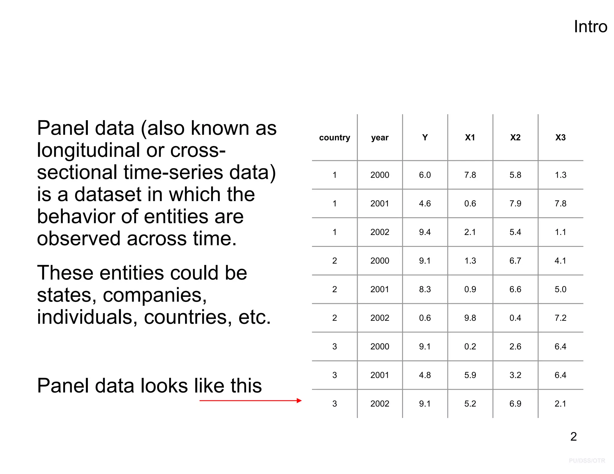
Intro
Panel data (also known as
longitudinal or cross-
sectional time-series data)
is a dataset in which the
behavior of entities are
observed across time.
These entities could be
states, companies,
individuals, countries, etc.
Panel data looks like this
country year Y X1 X2 X3
1 2000 6.0 7.8 5.8 1.3
1 2001 4.6 0.6 7.9 7.8
1 2002 9.4 2.1 5.4 1.1
2 2000 9.1 1.3 6.7 4.1
2 2001 8.3 0.9 6.6 5.0
2 2002 0.6 9.8 0.4 7.2
3 2000 9.1 0.2 2.6 6.4
3 2001 4.8 5.9 3.2 6.4
3 2002 9.1 5.2 6.9 2.1
2

PU/DSS/OTR
Intro
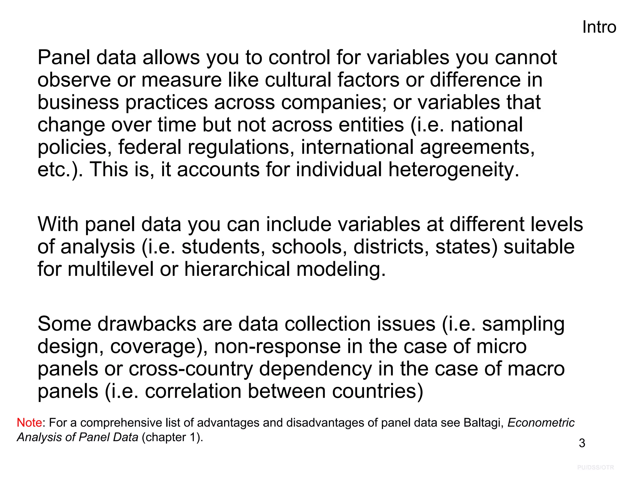
Panel data allows you to control for variables you cannot
observe or measure like cultural factors or difference in
business practices across companies; or variables that
change over time but not across entities (i.e. national
policies, federal regulations, international agreements,
etc.). This is, it accounts for individual heterogeneity.
With panel data you can include variables at different levels
of analysis (i.e. students, schools, districts, states) suitable
for multilevel or hierarchical modeling.
Some drawbacks are data collection issues (i.e. sampling
design, coverage), non-response in the case of micro
panels or cross-country dependency in the case of macro
panels (i.e. correlation between countries)
Note: For a comprehensive list of advantages and disadvantages of panel data see Baltagi, Econometric
Analysis of Panel Data (chapter 1). 3

PU/DSS/OTR
Intro
In this document we focus on two techniques
use to analyze panel data:
– Fixed effects
– Random effects
4

PU/DSS/OTR
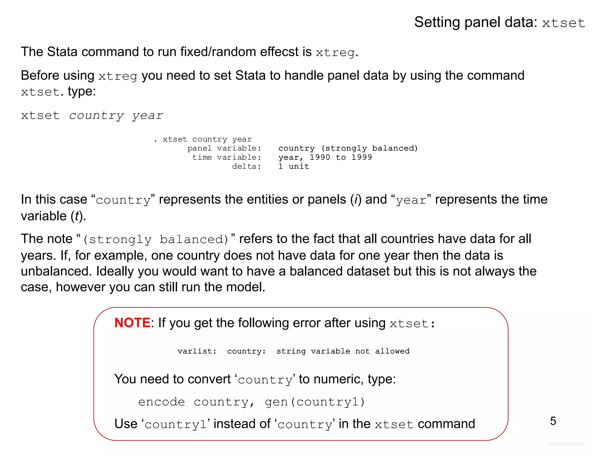
Setting panel data: xtset
The Stata command to run fixed/random effecst is xtreg.
Before using xtreg you need to set Stata to handle panel data by using the command
xtset. type:
xtset country year
delta: 1 unit
time variable: year, 1990 to 1999
panel variable: country (strongly balanced)
. xtset country year
In this case “country” represents the entities or panels (i) and “year” represents the time
variable (t).
The note “(strongly balanced)” refers to the fact that all countries have data for all
years. If, for example, one country does not have data for one year then the data is
unbalanced. Ideally you would want to have a balanced dataset but this is not always the
case, however you can still run the model.
NOTE: If you get the following error after using xtset:
You need to convert ‘country’ to numeric, type:
encode country, gen(country1)
Use ‘country1’ instead of ‘country’ in the xtset command 5
varlist: country: string variable not allowed

PU/DSS/OTR
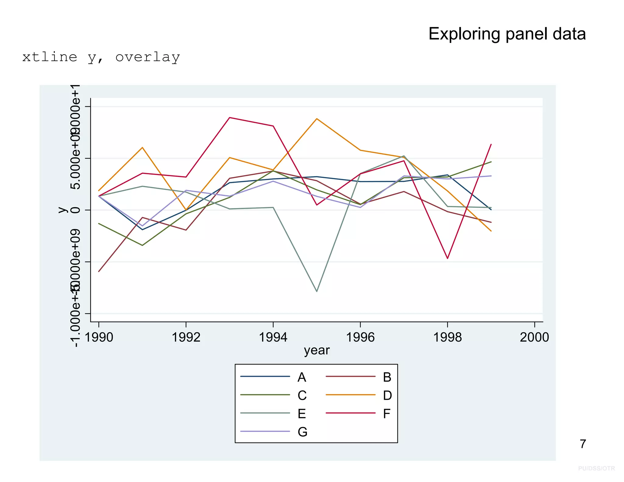
Exploring panel data
use http://dss.princeton.edu/training/Panel101.dta
xtset country year
xtline y
6
-1.000e+10
-5.000e+09
0
5.000e+09
1.000e+10
-1.000e+10
-5.000e+09
0
5.000e+09
1.000e+10
-1.000e+10
-5.000e+09
0
5.000e+09
1.000e+10
1990 1995 20001990 1995 2000
1990 1995 2000
A B C
D E F
G
y
year
Graphs by country

PU/DSS/OTR
Exploring panel data
xtline y, overlay
7
-1.000e+10
-5.000e+09
0
5.000e+09
1.000e+1
y
1990 1992 1994 1996 1998 2000
year
A B
C D
E F
G

PU/DSS/OTR
FIXED-EFFECTS MODEL
(Covariance Model, Within Estimator,
Individual Dummy Variable Model, Least
Squares Dummy Variable Model)
8

Fixed Effects
Use fixed-effects (FE) whenever you are only interested in analyzing the impact of
variables that vary over time.
FE explore the relationship between predictor and outcome variables within an entity
(country, person, company, etc.). Each entity has its own individual characteristics that
may or may not influence the predictor variables (for example, being a male or female
could influence the opinion toward certain issue; or the political system of a particular
country could have some effect on trade or GDP; or the business practices of a company
may influence its stock price).
When using FE we assume that something within the individual may impact or bias the
predictor or outcome variables and we need to control for this. This is the rationale behind
the assumption of the correlation between entity’s error term and predictor variables. FE
remove the effect of those time-invariant characteristics so we can assess the net effect of
the predictors on the outcome variable.
Another important assumption of the FE model is that those time-invariant characteristics
are unique to the individual and should not be correlated with other individual
characteristics. Each entity is different therefore the entity’s error term and the constant
(which captures individual characteristics) should not be correlated with the others. If the
error terms are correlated, then FE is no suitable since inferences may not be correct and
you need to model that relationship (probably using random-effects), this is the main
rationale for the Hausman test (presented later on in this document).
PU/DSS/OTR
9

PU/DSS/OTR
Fixed effects
The equation for the fixed effects model becomes:
Yit = β1Xit + αi + uit [eq.1]
Where
– αi (i=1….n) is the unknown intercept for each entity (n entity-specific intercepts).
– Yit is the dependent variable (DV) where i = entity and t = time.
– Xit represents one independent variable (IV),
– β1 is the coefficient for that IV,
– uit is the error term
“The key insight is that if the unobserved variable does not change over time, then any changes in
the dependent variable must be due to influences other than these fixed characteristics.” (Stock
and Watson, 2003, p.289-290).
“In the case of time-series cross-sectional data the interpretation of the beta coefficients would be
“…for a given country, as X varies across time by one unit, Y increases or decreases by β units”
(Bartels, Brandom, “Beyond “Fixed Versus Random Effects”: A framework for improving substantive and
statistical analysis of panel, time-series cross-sectional, and multilevel data”, Stony Brook University, working
paper, 2008).
Fixed-effects will not work well with data for which within-cluster variation is minimal or for slow
changing variables over time.
10

PU/DSS/OTR
Fixed effects
Another way to see the fixed effects model is by using binary variables. So the equation
for the fixed effects model becomes:
Yit = β0 + β1X1,it +…+ βkXk,it + γ2E2 +…+ γnEn + uit [eq.2]
Where
–Yit is the dependent variable (DV) where i = entity and t = time.
–Xk,it represents independent variables (IV),
–βk is the coefficient for the IVs,
–uit is the error term
–En is the entity n. Since they are binary (dummies) you have n-1 entities included in the model.
–γ2 Is the coefficient for the binary repressors (entities)
Both eq.1 and eq.2 are equivalents:
“the slope coefficient on X is the same from one [entity] to the next. The [entity]-specific
intercepts in [eq.1] and the binary regressors in [eq.2] have the same source: the unobserved
variable Zi that varies across states but not over time.” (Stock and Watson, 2003, p.280)
11

PU/DSS/OTR
Fixed effects
You could add time effects to the entity effects model to have a time and entity fixed
effects regression model:
Yit = β0 + β1X1,it +…+ βkXk,it + γ2E2 +…+ γnEn + δ2T2 +…+ δtTt + uit [eq.3]
Where
–Yit is the dependent variable (DV) where i = entity and t = time.
–Xk,it represents independent variables (IV),
–βk is the coefficient for the IVs,
–uit is the error term
–En is the entity n. Since they are binary (dummies) you have n-1 entities included in
the model.
–γ2 is the coefficient for the binary regressors (entities) .
–Tt is time as binary variable (dummy), so we have t-1 time periods.
–δ t is the coefficient for the binary time regressors .
Control for time effects whenever unexpected variation or special events my affect the
outcome variable.
12

PU/DSS/OTR
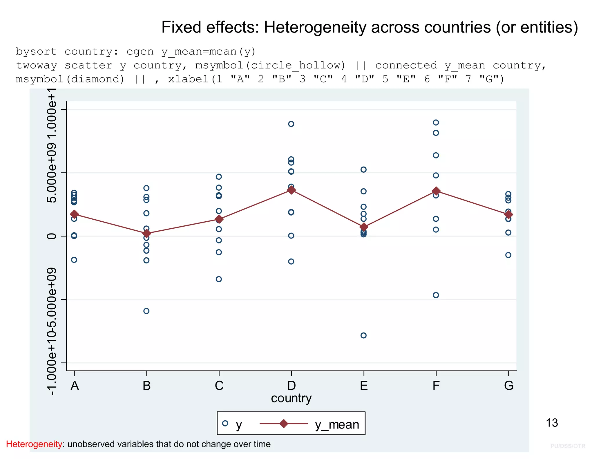
Fixed effects: Heterogeneity across countries (or entities)
bysort country: egen y_mean=mean(y)
twoway scatter y country, msymbol(circle_hollow) || connected y_mean country,
msymbol(diamond) || , xlabel(1 "A" 2 "B" 3 "C" 4 "D" 5 "E" 6 "F" 7 "G")
13
-1.000e+10-5.000e+09
0
5.000e+09
1.000e+1
A B C D E F G
country
y y_mean
Heterogeneity: unobserved variables that do not change over time

PU/DSS/OTR
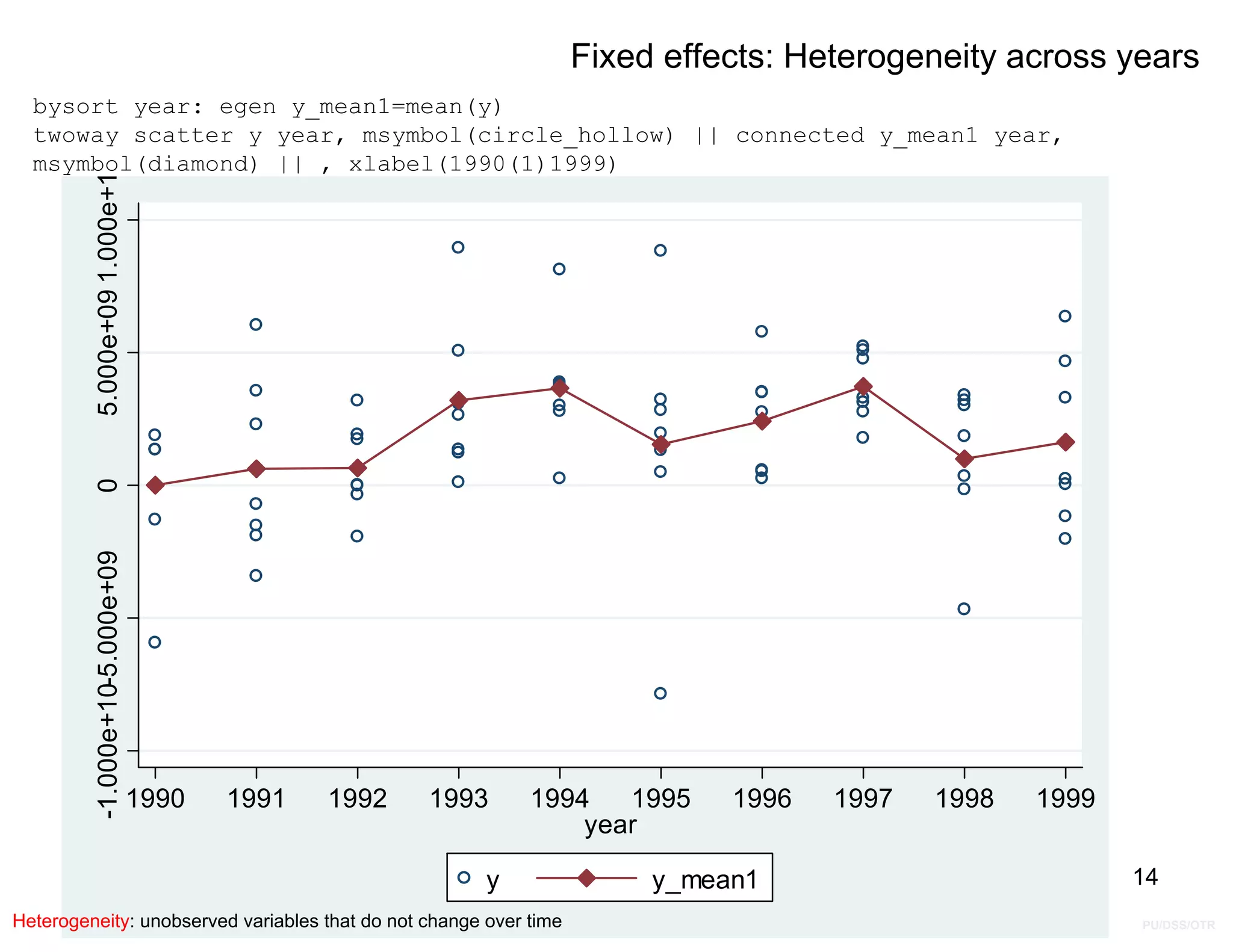
Fixed effects: Heterogeneity across years
bysort year: egen y_mean1=mean(y)
twoway scatter y year, msymbol(circle_hollow) || connected y_mean1 year,
msymbol(diamond) || , xlabel(1990(1)1999)
14
-1.000e+10-5.000e+09
0
5.000e+09
1.000e+1
1990 1991 1992 1993 1994 1995 1996 1997 1998 1999
year
y y_mean1
Heterogeneity: unobserved variables that do not change over time

PU/DSS/OTR
OLS regression
15
_cons 1.52e+09 6.21e+08 2.45 0.017 2.85e+08 2.76e+09
x1 4.95e+08 7.79e+08 0.64 0.527 -1.06e+09 2.05e+09
y Coef. Std. Err. t P>|t| [95% Conf. Interval]
Total 6.2729e+20 69 9.0912e+18 Root MSE = 3.0e+09
Adj R-squared = -0.0087
Residual 6.2359e+20 68 9.1705e+18 R-squared = 0.0059
Model 3.7039e+18 1 3.7039e+18 Prob > F = 0.5272
F( 1, 68) = 0.40
Source SS df MS Number of obs = 70
. regress y x1
A
A
A
A A A
A
A
A
A
B
B
B
B
B
B
B
B
B
B C
C
C
C
C
C
C
C
C
C
D
D
D
D
D
D
D
D
D
D
E
E
E
E E
E
E
E
E
E
F
F F
F
F
F
F
F
F
F
G
G
G
G
G
G
G
G
G
G
-1.000e+10-5.000e+09
0
5.000e+09
1.000e+1
-.5 0 .5 1 1.5
x1
y Fitted values
twoway scatter y x1,
mlabel(country) || lfit y x1,
clstyle(p2)

PU/DSS/OTR
Fixed Effects using least
squares dummy variable
model (LSDV)
.
16
_cons 8.81e+08 9.62e+08 0.92 0.363 -1.04e+09 2.80e+09
_Icountry_7 -1.87e+09 1.50e+09 -1.25 0.218 -4.86e+09 1.13e+09
_Icountry_6 1.13e+09 1.29e+09 0.88 0.384 -1.45e+09 3.71e+09
_Icountry_5 -1.48e+09 1.27e+09 -1.17 0.247 -4.02e+09 1.05e+09
_Icountry_4 2.28e+09 1.26e+09 1.81 0.075 -2.39e+08 4.80e+09
_Icountry_3 -2.60e+09 1.60e+09 -1.63 0.108 -5.79e+09 5.87e+08
_Icountry_2 -1.94e+09 1.26e+09 -1.53 0.130 -4.47e+09 5.89e+08
x1 2.48e+09 1.11e+09 2.24 0.029 2.63e+08 4.69e+09
Adj R-squared = 0.1404
Model 1.4276e+20 7 2.0394e+19 Prob > F = 0.0199
F( 7, 62) = 2.61
i.country _Icountry_1-7 (naturally coded; _Icountry_1 omitted)
. xi: regress y x1 i.country
-2.00e+09
0
2.00e+09
4.00e+09
6.00e+09
-.5 0 .5 1 1.5
x1
yhat, country == A yhat, country == B
yhat, country == C yhat, country == D
yhat, country == E yhat, country == F
yhat, country == G Fitted values
xi: regress y x1 i.country
predict yhat
separate y, by(country)
separate yhat, by(country)
twoway connected yhat1-yhat7
x1, msymbol(none
diamond_hollow triangle_hollow
square_hollow + circle_hollow
x) msize(medium) mcolor(black
black black black black black
black) || lfit y x1,
clwidth(thick) clcolor(black)
OLS regression
NOTE: In Stata 11 you do not need
“xi:” when adding dummy variables

PU/DSS/OTR
Fixed effects
The least square dummy variable model (LSDV) provides a good way to understand fixed
effects.
The effect of x1 is mediated by the differences across countries.
By adding the dummy for each country we are estimating the pure effect of x1 (by
controlling for the unobserved heterogeneity).
Each dummy is absorbing the effects particular to each country.
17
regress y x1
estimates store ols
xi: regress y x1 i.country
estimates store ols_dum
estimates table ols ols_dum, star stats(N)
legend: * p<0.05; ** p<0.01; *** p<0.001
N 70 70
_cons 1.524e+09* 8.805e+08
_Icountry_7 -1.865e+09
_Icountry_6 1.130e+09
x1 4.950e+08 2.476e+09*
Variable ols ols_dum
. estimates table ols ols_dum, star stats(N)

PU/DSS/OTR
Fixed effects: n entity-specific intercepts using xtreg
Comparing the fixed effects using dummies with xtreg we get the same results.
18
rho .29726926 (fraction of variance due to u_i)
sigma_e 2.796e+09
sigma_u 1.818e+09
_cons 2.41e+08 7.91e+08 0.30 0.762 -1.34e+09 1.82e+09
x1 2.48e+09 1.11e+09 2.24 0.029 2.63e+08 4.69e+09
corr(u_i, Xb) = -0.5468 Prob > F = 0.0289
F(1,62) = 5.00
overall = 0.0059 max = 10
between = 0.0763 avg = 10.0
R-sq: within = 0.0747 Obs per group: min = 10
Group variable: country Number of groups = 7
Fixed-effects (within) regression Number of obs = 70
. xtreg y x1, fe
_cons 8.81e+08 9.62e+08 0.92 0.363 -1.04e+09 2.80e+09
_Icountry_7 -1.87e+09 1.50e+09 -1.25 0.218 -4.86e+09 1.13e+09
_Icountry_6 1.13e+09 1.29e+09 0.88 0.384 -1.45e+09 3.71e+09
_Icountry_5 -1.48e+09 1.27e+09 -1.17 0.247 -4.02e+09 1.05e+09
_Icountry_4 2.28e+09 1.26e+09 1.81 0.075 -2.39e+08 4.80e+09
_Icountry_3 -2.60e+09 1.60e+09 -1.63 0.108 -5.79e+09 5.87e+08
_Icountry_2 -1.94e+09 1.26e+09 -1.53 0.130 -4.47e+09 5.89e+08
x1 2.48e+09 1.11e+09 2.24 0.029 2.63e+08 4.69e+09
Model 1.4276e+20 7 2.0394e+19 Prob > F = 0.0199
F( 7, 62) = 2.61
OLS regression
Using xtreg

PU/DSS/OTR
Fixed effects option
sigma_e 2.796e+09
sigma_u 1.818e+09
_cons 2.41e+08 7.91e+08 0.30 0.762 -1.34e+09 1.82e+09
x1 2.48e+09 1.11e+09 2.24 0.029 2.63e+08 4.69e+09
corr(u_i, Xb) = -0.5468 Prob > F = 0.0289
F(1,62) = 5.00
between = 0.0763 avg = 10.0
. xtreg y x1, fe
Fixed effects: n entity-specific intercepts (using xtreg)
Outcome
variable
Predictor
variable(s)
Yit = β1Xit +…+ βkXkt + αi + eit [see eq.1]
Total number of cases (rows)
Total number of groups
(entities)
If this number is < 0.05 then
your model is ok. This is a
test (F) to see whether all the
coefficients in the model are
different than zero.
Two-tail p-values test the
hypothesis that each
coefficient is different from 0.
To reject this, the p-value has
to be lower than 0.05 (95%,
you could choose also an
alpha of 0.10), if this is the
case then you can say that the
variable has a significant
influence on your dependent
variable (y)
t-values test the hypothesis that each coefficient is
different from 0. To reject this, the t-value has to
be higher than 1.96 (for a 95% confidence). If this
is the case then you can say that the variable has
a significant influence on your dependent variable
(y). The higher the t-value the higher the
relevance of the variable.
Coefficients of the
regressors. Indicate how
much Y changes when X
increases by one unit.
29.7% of the variance is
due to differences
across panels.
‘rho’ is known as the
intraclass correlation
The errors ui
are correlated
with the
regressors in
the fixed effects
model
2
2
2
)
_
(
)
_
(
)
_
(
e
sigma
u
sigma
u
sigma
rho


sigma_u = sd of residuals within groups ui
sigma_e = sd of residuals (overall error term) ei
For more info see Hamilton, Lawrence,
Statistics with STATA.
19
NOTE: Add the option ‘robust’ to control for heteroskedasticity

PU/DSS/OTR
country F(6, 62) = 2.965 0.013 (7 categories)
_cons 2.41e+08 7.91e+08 0.30 0.762 -1.34e+09 1.82e+09
x1 2.48e+09 1.11e+09 2.24 0.029 2.63e+08 4.69e+09
Root MSE = 2.8e+09
R-squared = 0.2276
Prob > F = 0.0289
F( 1, 62) = 5.00
Linear regression, absorbing indicators Number of obs = 70
. areg y x1, absorb(country)
Another way to estimate fixed effects:
n entity-specific intercepts
(using areg)
Outcome
variable Predictor
variable(s)
Hide the binary variables for each entity
Yit = β1Xit +…+ βkXkt + αi + eit [see eq.1]
variable (y)
Coefficients of the
regressors. Indicate how
much Y changes when X
increases by one unit.
R-square shows the amount
of variance of Y explained by
X
Adj R-square shows the
same as R-sqr but adjusted
by the number of cases and
number of variables. When
the number of variables is
small and the number of
cases is very large then Adj
R-square is closer to R-
square.
“Although its output is less informative than regression
with explicit dummy variables, areg does have two
advantages. It speeds up exploratory work, providing
quick feedback about whether a dummy variable
approach is worthwhile. Secondly, when the variable of
interest has many values, creating dummies for each of
them could lead to too many variables or too large a
model ….” (Hamilton, 2006, p.180) 20

PU/DSS/OTR
_cons 8.81e+08 9.62e+08 0.92 0.363 -1.04e+09 2.80e+09
_Icountry_7 -1.87e+09 1.50e+09 -1.25 0.218 -4.86e+09 1.13e+09
_Icountry_6 1.13e+09 1.29e+09 0.88 0.384 -1.45e+09 3.71e+09
_Icountry_5 -1.48e+09 1.27e+09 -1.17 0.247 -4.02e+09 1.05e+09
_Icountry_4 2.28e+09 1.26e+09 1.81 0.075 -2.39e+08 4.80e+09
_Icountry_3 -2.60e+09 1.60e+09 -1.63 0.108 -5.79e+09 5.87e+08
_Icountry_2 -1.94e+09 1.26e+09 -1.53 0.130 -4.47e+09 5.89e+08
x1 2.48e+09 1.11e+09 2.24 0.029 2.63e+08 4.69e+09
Model 1.4276e+20 7 2.0394e+19 Prob > F = 0.0199
F( 7, 62) = 2.61
Another way to estimate fixed effects: common intercept
and n-1 binary regressors (using dummies and regress)
R-square shows the amount
of variance of Y explained by
X
variable (y)
Coefficients of
the regressors
indicate how
much Y
changes
when X
increases by
one unit.
Outcome
variable
Predictor
variable(s) Notice the “i.” before the indicator variable for entities
Notice the “xi:”
(interaction expansion)
to automatically
generate dummy
variables
21
NOTE: In Stata 11 you do not need
“xi:” when adding dummy variables

PU/DSS/OTR
Fixed effects: comparing xtreg (with fe), regress (OLS with dummies) and areg
To compare the previous methods type “estimates store [name]” after running each regression, at
the end use the command “estimates table…” (see below):
xtreg y x1 x2 x3, fe
estimates store fixed
xi: regress y x1 x2 x3 i.country
estimates store ols
areg y x1 x2 x3, absorb(country)
estimates store areg
estimates table fixed ols areg, star stats(N r2 r2_a)
All three commands provide the same
results
Tip: When reporting the R-square use
the one provided by either regress
or areg.
22
legend: * p<0.05; ** p<0.01; *** p<0.001
r2_a -.03393692 .13690428 .13690428
r2 .10092442 .24948198 .24948198
N 70 70 70
_cons -2.060e+08 2.073e+09 -2.060e+08
x3 3.097e+08 3.097e+08 3.097e+08
x2 1.823e+09 1.823e+09 1.823e+09
x1 2.425e+09* 2.425e+09* 2.425e+09*
Variable fixed ols areg
. estimates table fixed ols areg, star stats(N r2 r2_a)

PU/DSS/OTR
A note on fixed-effects…
“…The fixed-effects model controls for all time-invariant
differences between the individuals, so the estimated
coefficients of the fixed-effects models cannot be biased
because of omitted time-invariant characteristics…[like culture,
religion, gender, race, etc]
One side effect of the features of fixed-effects models is that
they cannot be used to investigate time-invariant causes of the
dependent variables. Technically, time-invariant characteristics
of the individuals are perfectly collinear with the person [or
entity] dummies. Substantively, fixed-effects models are
designed to study the causes of changes within a person [or
entity]. A time-invariant characteristic cannot cause such a
change, because it is constant for each person.” (Underline is
mine) Kohler, Ulrich, Frauke Kreuter, Data Analysis Using
Stata, 2nd ed., p.245 23

PU/DSS/OTR
RANDOM-EFFECTS MODEL
(Random Intercept, Partial Pooling
Model)
24

PU/DSS/OTR
Random effects
The rationale behind random effects model is that, unlike the fixed effects model,
the variation across entities is assumed to be random and uncorrelated with the
predictor or independent variables included in the model:
“…the crucial distinction between fixed and random effects is whether the unobserved
individual effect embodies elements that are correlated with the regressors in the
model, not whether these effects are stochastic or not” [Green, 2008, p.183]
If you have reason to believe that differences across entities have some influence
on your dependent variable then you should use random effects.
An advantage of random effects is that you can include time invariant variables (i.e.
gender). In the fixed effects model these variables are absorbed by the intercept.
The random effects model is:
Yit = βXit + α + uit + εit [eq.4]
25
Within-entity error
Between-entity error

PU/DSS/OTR
Random effects
Random effects assume that the entity’s error term is not correlated with the
predictors which allows for time-invariant variables to play a role as explanatory
variables.
In random-effects you need to specify those individual characteristics that may or
may not influence the predictor variables. The problem with this is that some
variables may not be available therefore leading to omitted variable bias in the
model.
RE allows to generalize the inferences beyond the sample used in the model.
26

PU/DSS/OTR
sigma_e 2.796e+09
sigma_u 1.065e+09
_cons 1.04e+09 7.91e+08 1.31 0.190 -5.13e+08 2.59e+09
x1 1.25e+09 9.02e+08 1.38 0.167 -5.21e+08 3.02e+09
y Coef. Std. Err. z P>|z| [95% Conf. Interval]
corr(u_i, X) = 0 (assumed) Prob > chi2 = 0.1669
Random effects u_i ~ Gaussian Wald chi2(1) = 1.91
between = 0.0763 avg = 10.0
Random-effects GLS regression Number of obs = 70
. xtreg y x1, re
Random effects
You can estimate a random effects model using xtreg and the option re.
Outcome
variable
Predictor
variable(s)
Random effects
option
Differences
across units
are
uncorrelated
with the
regressors
If this number is < 0.05
then your model is ok.
This is a test (F) to see
whether all the
coefficients in the
model are different
than zero.
Two-tail p-values test
the hypothesis that each
coefficient is different
from 0. To reject this, the
p-value has to be lower
than 0.05 (95%, you
could choose also an
alpha of 0.10), if this is
the case then you can
say that the variable has
a significant influence on
your dependent variable
(y)
27
Interpretation of the coefficients is tricky since they include both the within-entity and between-entity effects.
In the case of TSCS data represents the average effect of X over Y when X changes across time and
between countries by one unit.

PU/DSS/OTR
FIXED OR RANDOM?
28

PU/DSS/OTR
Prob>chi2 = 0.0553
= 3.67
chi2(1) = (b-B)'[(V_b-V_B)^(-1)](b-B)
Test: Ho: difference in coefficients not systematic
B = inconsistent under Ha, efficient under Ho; obtained from xtreg
b = consistent under Ho and Ha; obtained from xtreg
x1 2.48e+09 1.25e+09 1.23e+09 6.41e+08
fixed random Difference S.E.
(b) (B) (b-B) sqrt(diag(V_b-V_B))
Coefficients
. hausman fixed random
If this is < 0.05 (i.e. significant) use fixed effects.
Fixed or Random: Hausman test
xtreg y x1, fe
estimates store fixed
xtreg y x1, re
estimates store random
hausman fixed random
To decide between fixed or random effects you can run a Hausman test where the
null hypothesis is that the preferred model is random effects vs. the alternative the
fixed effects (see Green, 2008, chapter 9). It basically tests whether the unique
errors (ui) are correlated with the regressors, the null hypothesis is they are not.
Run a fixed effects model and save the estimates, then run a random model and
save the estimates, then perform the test. See below.
29

PU/DSS/OTR
OTHER TESTS/
DIAGNOSTICS
30

Testing for time-fixed effects
To see if time fixed effects are needed
when running a FE model use the
command testparm. It is a joint test to
see if the dummies for all years are equal
to 0, if they are then no time fixed effects
are needed (type help testparm for
more details)
After running the fixed effect model, type:
testparm i.year
NOTE: If using Stata 10 or older type
xi: xtreg y x1 i.year, fe
testparm _Iyear*
Prob > F = 0.3094
F( 9, 53) = 1.21
( 9) 1999.year = 0
( 8) 1998.year = 0
( 7) 1997.year = 0
( 6) 1996.year = 0
( 5) 1995.year = 0
( 4) 1994.year = 0
( 3) 1993.year = 0
( 2) 1992.year = 0
( 1) 1991.year = 0
. testparm i.year
F test that all u_i=0: F(6, 53) = 2.45 Prob > F = 0.0362
sigma_e 2.754e+09
sigma_u 1.547e+09
_cons -3.98e+08 1.11e+09 -0.36 0.721 -2.62e+09 1.83e+09
1999 1.26e+09 1.51e+09 0.83 0.409 -1.77e+09 4.29e+09
1998 3.67e+08 1.59e+09 0.23 0.818 -2.82e+09 3.55e+09
1997 2.99e+09 1.63e+09 1.84 0.072 -2.72e+08 6.26e+09
1996 1.67e+09 1.63e+09 1.03 0.310 -1.60e+09 4.95e+09
1995 9.74e+08 1.57e+09 0.62 0.537 -2.17e+09 4.12e+09
1994 2.85e+09 1.66e+09 1.71 0.092 -4.84e+08 6.18e+09
1993 2.87e+09 1.50e+09 1.91 0.061 -1.42e+08 5.89e+09
1992 1.45e+08 1.55e+09 0.09 0.925 -2.96e+09 3.25e+09
1991 2.96e+08 1.50e+09 0.20 0.844 -2.72e+09 3.31e+09
year
x1 1.39e+09 1.32e+09 1.05 0.297 -1.26e+09 4.04e+09
corr(u_i, Xb) = -0.2014 Prob > F = 0.1311
F(10,53) = 1.60
between = 0.0763 avg = 10.0
. xtreg y x1 i.year, fe
The Prob>F is > 0.05, so we
failed to reject the null that the
coefficients for all years are jointly
equal to zero, therefore no time fixed-
effects are needed in this case.
PU/DSS/OTR
31

PU/DSS/OTR
Testing for random effects: Breusch-Pagan Lagrange multiplier (LM)
The LM test helps you decide between a random effects regression and a simple
OLS regression.
The null hypothesis in the LM test is that variances across entities is zero. This is,
no significant difference across units (i.e. no panel effect). The command in Stata
is xttset0 type it right after running the random effects model.
32
xtreg y x1, re
xttest0
Prob > chi2 = 0.1023
chi2(1) = 2.67
Test: Var(u) = 0
u 1.13e+18 1.06e+09
e 7.82e+18 2.80e+09
y 9.09e+18 3.02e+09
Var sd = sqrt(Var)
Estimated results:
y[country,t] = Xb + u[country] + e[country,t]
Breusch and Pagan Lagrangian multiplier test for random effects
. xttest0
Here we failed to reject the null and conclude that random effects is not appropriate. This is, no
evidence of significant differences across countries, therefore you can run a simple OLS
regression.

PU/DSS/OTR
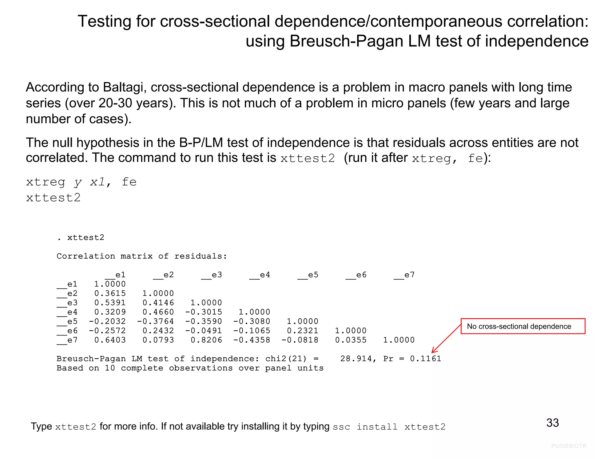
Testing for cross-sectional dependence/contemporaneous correlation:
using Breusch-Pagan LM test of independence
According to Baltagi, cross-sectional dependence is a problem in macro panels with long time
series (over 20-30 years). This is not much of a problem in micro panels (few years and large
number of cases).
The null hypothesis in the B-P/LM test of independence is that residuals across entities are not
correlated. The command to run this test is xttest2 (run it after xtreg, fe):
xtreg y x1, fe
xttest2
33
No cross-sectional dependence
Based on 10 complete observations over panel units
Breusch-Pagan LM test of independence: chi2(21) = 28.914, Pr = 0.1161
__e7 0.6403 0.0793 0.8206 -0.4358 -0.0818 0.0355 1.0000
__e6 -0.2572 0.2432 -0.0491 -0.1065 0.2321 1.0000
__e5 -0.2032 -0.3764 -0.3590 -0.3080 1.0000
__e4 0.3209 0.4660 -0.3015 1.0000
__e3 0.5391 0.4146 1.0000
__e2 0.3615 1.0000
__e1 1.0000
__e1 __e2 __e3 __e4 __e5 __e6 __e7
Correlation matrix of residuals:
. xttest2
Type xttest2 for more info. If not available try installing it by typing ssc install xttest2

PU/DSS/OTR
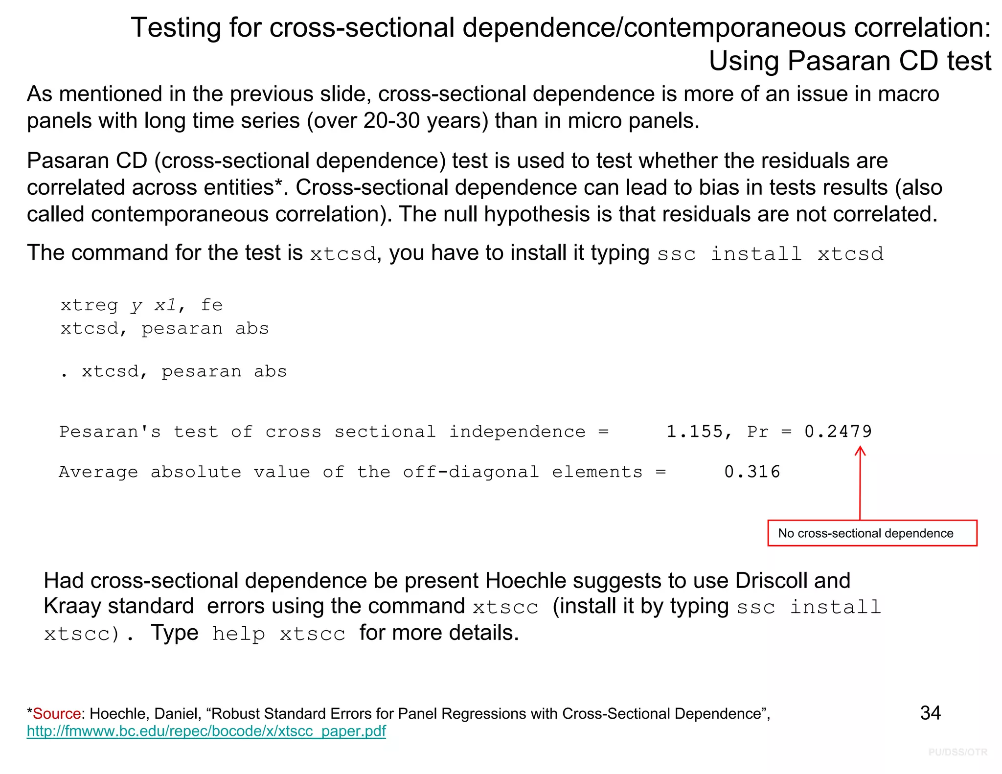
Testing for cross-sectional dependence/contemporaneous correlation:
Using Pasaran CD test
xtreg y x1, fe
xtcsd, pesaran abs
As mentioned in the previous slide, cross-sectional dependence is more of an issue in macro
panels with long time series (over 20-30 years) than in micro panels.
Pasaran CD (cross-sectional dependence) test is used to test whether the residuals are
correlated across entities*. Cross-sectional dependence can lead to bias in tests results (also
called contemporaneous correlation). The null hypothesis is that residuals are not correlated.
The command for the test is xtcsd, you have to install it typing ssc install xtcsd
34
Average absolute value of the off-diagonal elements = 0.316
Pesaran's test of cross sectional independence = 1.155, Pr = 0.2479
. xtcsd, pesaran abs
No cross-sectional dependence
Had cross-sectional dependence be present Hoechle suggests to use Driscoll and
Kraay standard errors using the command xtscc (install it by typing ssc install
xtscc). Type help xtscc for more details.
*Source: Hoechle, Daniel, “Robust Standard Errors for Panel Regressions with Cross-Sectional Dependence”,
http://fmwww.bc.edu/repec/bocode/x/xtscc_paper.pdf

Testing for heteroskedasticity
A test for heteroskedasticiy is avalable for the fixed- effects model using the command
xttest3.
This is a user-written program, to install it type:
ssc install xtest3
xttest3
.xttest3
Modified Wald test for groupwise heteroskedasticity
in fixed effect regression model
H0: sigma(i)^2 = sigma^2 for all i
chi2 (7) = 42.77
Prob>chi2 = 0.0000
The null is homoskedasticity (or constant variance). Above we reject the null and conclude
heteroskedasticity. Type help xttest3 for more details.
NOTE: Use the option ‘robust’ to obtain heteroskedasticity-robust standard errors (also
known as Huber/White or sandwich estimators).
Presence of heteroskedasticity
PU/DSS/OTR
35

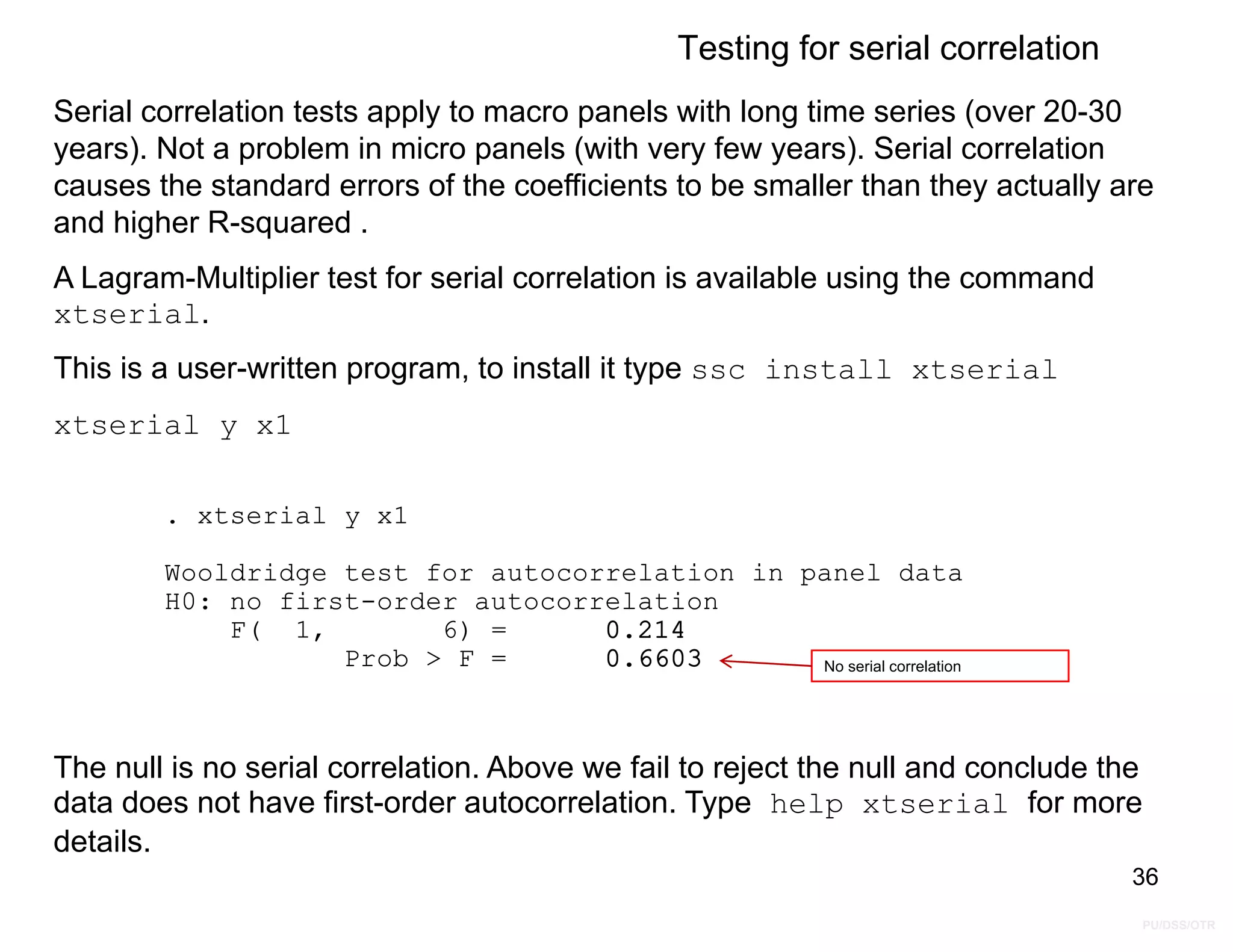
PU/DSS/OTR
Prob > F = 0.6603
F( 1, 6) = 0.214
H0: no first-order autocorrelation
Wooldridge test for autocorrelation in panel data
. xtserial y x1
Testing for serial correlation
Serial correlation tests apply to macro panels with long time series (over 20-30
years). Not a problem in micro panels (with very few years). Serial correlation
causes the standard errors of the coefficients to be smaller than they actually are
and higher R-squared .
A Lagram-Multiplier test for serial correlation is available using the command
xtserial.
This is a user-written program, to install it type ssc install xtserial
xtserial y x1
36
No serial correlation
The null is no serial correlation. Above we fail to reject the null and conclude the
data does not have first-order autocorrelation. Type help xtserial for more
details.

PU/DSS/OTR
Testing for unit roots/stationarity
Stata 11 has a series of unit root tests using the command xtunitroot, it
included the following series of tests (type help xtunitroot for more info on
how to run the tests):
“xtunitroot performs a variety of tests for unit roots (or stationarity) in panel datasets. The Levin-Lin-Chu
(2002), Harris-Tzavalis (1999), Breitung (2000; Breitung and Das 2005), Im-Pesaran-Shin (2003), and
Fisher-type (Choi 2001) tests have as the null hypothesis that all the panels contain a unit root. The Hadri
(2000) Lagrange multiplier (LM) test has as the null hypothesis that all the panels are (trend) stationary.
The top of the output for each test makes explicit the null and alternative hypotheses. Options allow you to
include panel-specific means (fixed effects) and time trends in the model of the data-generating process”
[Source: http://www.stata.com/help.cgi?xtunitroot or type help xtunitroot]
Stata 10 does not have this command but can run user-written programs to run the
same tests. You will have to find them and install them in your Stata program
(remember, these are only for Stata 9.2/10). To find the add-ons type:
findit panel unit root test
A window will pop-up, find the desired test, click on the blue link, then click where it
says “(click here to install)”
For more info on unit roots please check: http://dss.princeton.edu/training/TS101.pdf
37

PU/DSS/OTR
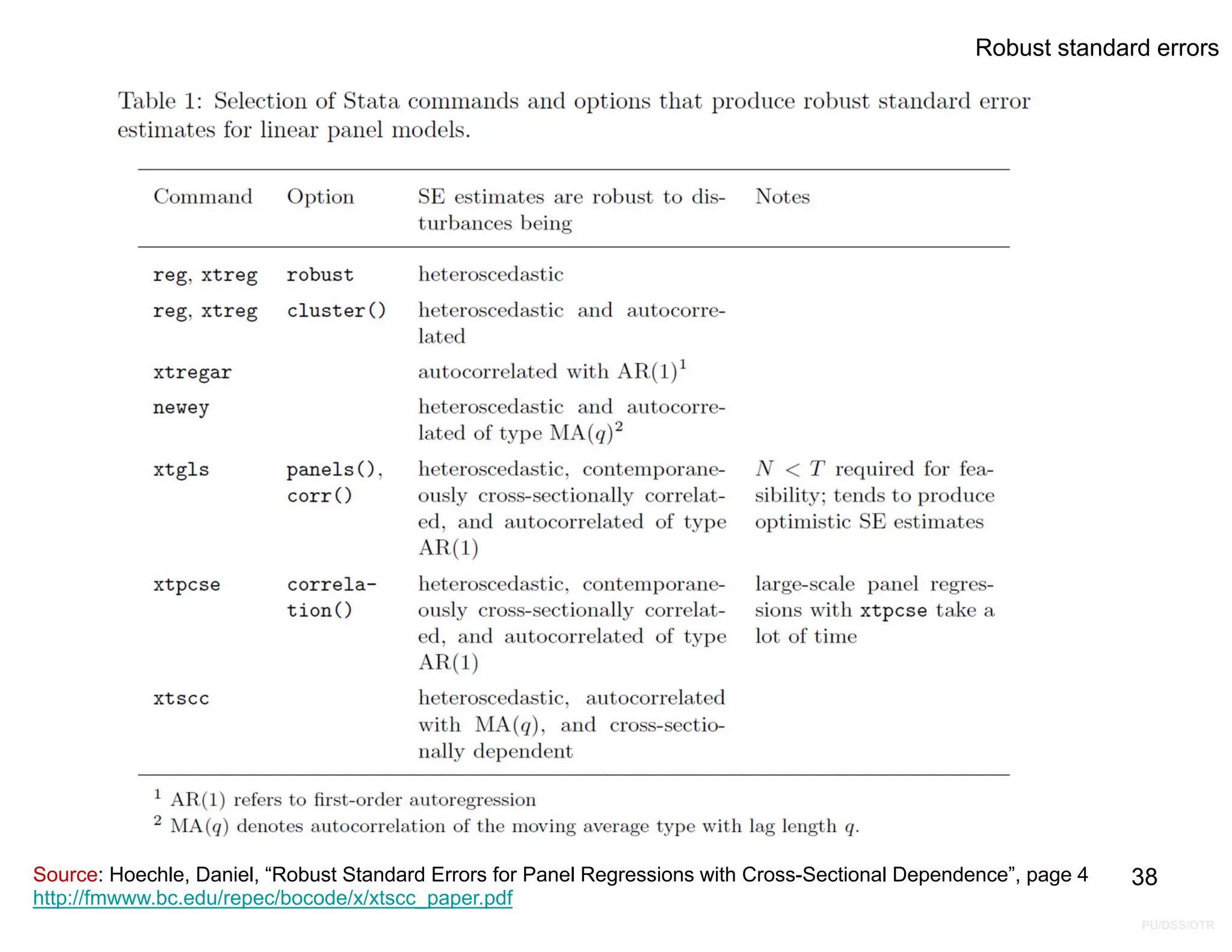
Robust standard errors
38
Source: Hoechle, Daniel, “Robust Standard Errors for Panel Regressions with Cross-Sectional Dependence”, page 4

PU/DSS/OTR
Summary of basic models (FE/RE)
Command Syntax
Entity fixed effects
xtreg xtreg y x1 x2 x3 x4 x5 x6 x7, fe
areg areg y x1 x2 x3 x4 x5 x6 x7, absorb(country)
regress xi: regress y x1 x2 x3 x4 x5 x6 x7 i.country,
Entity and time fixed effects
xi: xtreg xi: xtreg y x1 x2 x3 x4 x5 x6 x7 i.year, fe
xi: areg xi: areg y x1 x2 x3 x4 x5 x6 x7 i.year, absorb(country)
xi: regress xi: regress y x1 x2 x3 x4 x5 x6 x7 i.country i.year
Random effects
xtreg xtreg y x1 x2 x3 x4 x5 x6 x7, re robust
39
NOTE: In Stata 11 you do not need “xi:” when adding dummy variables using regress or areg

PU/DSS/OTR
40
Useful links / Recommended books / References
• DSS Online Training Section http://dss.princeton.edu/training/
• UCLA Resources http://www.ats.ucla.edu/stat/
• Princeton DSS Libguides http://libguides.princeton.edu/dss
Books/References
• “Beyond “Fixed Versus Random Effects”: A framework for improving substantive and statistical
analysis of panel, time-series cross-sectional, and multilevel data” / Brandom Bartels
http://polmeth.wustl.edu/retrieve.php?id=838
• “Robust Standard Errors for Panel Regressions with Cross-Sectional Dependence” / Daniel Hoechle,
• An Introduction to Modern Econometrics Using Stata/ Christopher F. Baum, Stata Press, 2006.
• Data analysis using regression and multilevel/hierarchical models / Andrew Gelman, Jennifer Hill.
Cambridge ; New York : Cambridge University Press, 2007.
• Data Analysis Using Stata/ Ulrich Kohler, Frauke Kreuter, 2nd ed., Stata Press, 2009.
• Designing Social Inquiry: Scientific Inference in Qualitative Research / Gary King, Robert O.
Keohane, Sidney Verba, Princeton University Press, 1994.
• Econometric analysis / William H. Greene. 6th ed., Upper Saddle River, N.J. : Prentice Hall, 2008.
• Econometric Analysis of Panel Data, Badi H. Baltagi, Wiley, 2008
• Introduction to econometrics / James H. Stock, Mark W. Watson. 2nd ed., Boston: Pearson Addison
Wesley, 2007.
• Statistical Analysis: an interdisciplinary introduction to univariate & multivariate methods / Sam
Kachigan, New York : Radius Press, c1986
• Statistics with Stata (updated for version 9) / Lawrence Hamilton, Thomson Books/Cole, 2006
• Unifying Political Methodology: The Likelihood Theory of Statistical Inference / Gary King, Cambridge
University Press, 1989

Panel101.pdf

In this document

More Related Content

What's hot

Similar to Panel101.pdf

Recently uploaded

Panel101.pdf