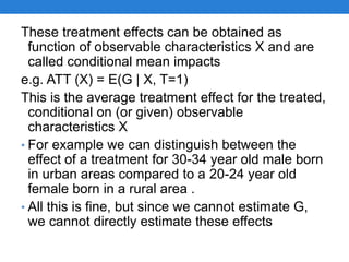
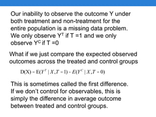
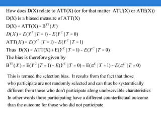
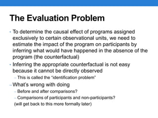
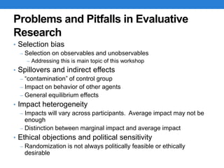
This document discusses causal inference and program evaluation. It notes that evaluating programs requires estimating the counterfactual outcome for participants in the absence of the program, which is difficult. Common problems in evaluation include selection bias if participants differ from non-participants in unobserved ways, spillover effects, and impact heterogeneity. Internal validity assesses if the true impact is measured, while external validity examines generalizability. Estimating average treatment effects requires addressing non-random selection into programs.

1. Causal Inference and
Program Evaluation
Day 1, Lecture 1
By Ragui Assaad
Training on Applied Micro-Econometrics and Public Policy
Evaluation
July 25-27, 2016
Economic Research Forum

2. Readings
• Ravallion, Martin (2008). “Evaluation in the Practice of
Development.” Policy Research Working Paper 4547,
Development Research Group, the World Bank,
Washington DC.
• And
• Ravallion, Martin (2008) “Evaluating Anti-Poverty
Programs” in Handbook of Development Economics, Ch.
59. Vol. 4. Amsterdam: Elsevier.

3. The Evaluation Problem
• To determine the causal effect of programs assigned
exclusively to certain observational units, we need to
estimate the impact of the program on participants by
inferring what would have happened in the absence of the
program (the counterfactual)
• Inferring the appropriate counterfactual is not easy
because it cannot be directly observed
– This is called the “identification problem”
–What’s wrong with doing
– Before and after comparisons?
– Comparisons of participants and non-participants?
(will get back to this more formally later)

4. Evaluative Research
• What is evaluative research
• Ex ante: project appraisal or cost-benefit analysis
• Ex post: process and impact evaluation

5. Problems and Pitfalls in Evaluative
Research
• Selection bias
– Selection on observables and unobservables
– Addressing this is main topic of this workshop
• Spillovers and indirect effects
– “contamination” of control group
– Impact on behavior of other agents
– General equilibrium effects
• Impact heterogeneity
– Impacts will vary across participants. Average impact may not be
enough
– Distinction between marginal impact and average impact
• Ethical objections and political sensitivity
– Randomization is not always politically feasible or ethically
desirable

6. Internal and External Validity
• Internal validity
– Are we measuring the true impact of the intervention in this setting?
• External validity
– How does this conclusion generalize to other settings?
– What lessons do we learn for future policies?
– Will need to know why an impact is obtained and not just whether
there is an impact
– Understanding the influence of context is crucial to external validity

7. Understanding Impact
• What factors influence measured outcomes?
– What factors affect who participates and who doesn’t?
– How do participants’ characteristics affect the outcome?
– How do quality/quantity of service provision or the nature of local
institutions affect outcomes? (context)
• Assessing impact on intermediate outcome measures,
like behavior of program participants
• Full impact may not occur within relevant time period

8. Back to the Evaluation Problem: A
Statistical Formulation
• Y is observable outcome of interest
• Impact of program is the change in Y over relevant time
period where impact is expected and that can be causally
attributed to program
ttreatmenreceivingnotoftualcounterfacunderiindividualforoutcomeis
eatmentunder triindividualforoutcomeis
notortreated""wasiindividualwhetherindicatingabledummy variais
iindividualforoutcomeis
C
i
T
i
i
i
Y
Y
T
Y
C
i
T
ii YYG 
:bygivenisiunitoneffectcausalorimpactgain,The

9. • Focus here will be on measuring average impact
• Average Treatment Effect (ATE) = E(G)
Where E is the expectation operator. You can think
of it as the “average” function across individuals.
Read: Expected value of G
• Because of selection, the average treatment effect
can be different for the treated and the untreated.
• The treated group is different from the untreated
group along unobservable characteristics

10. ATT = E(G |T=1) is the average treatment effect of the
treated (sometimes called TT)
Read: Expected value of G given than individuals (over
whom the average is taken) were treated
This is the expected impact of the treatment on those who
actually participated in program.

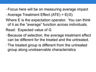
11. ATU = E(G | T=0) is the average treatment effect on the
untreated (sometimes called TU)
This is the expected impact of the treatment on those who
did not participate.
Thus the average treatment effect for a random individual
in the population is given by
ATE = ATT * Pr[T=1] + ATU * Pr[T=0]
where Pr[T=1] is the probability of being treated.

12. These treatment effects can be obtained as
function of observable characteristics X and are
called conditional mean impacts
e.g. ATT (X) = E(G | X, T=1)
This is the average treatment effect for the treated,
conditional on (or given) observable
characteristics X
• For example we can distinguish between the
effect of a treatment for 30-34 year old male born
in urban areas compared to a 20-24 year old
female born in a rural area .
• All this is fine, but since we cannot estimate G,
we cannot directly estimate these effects

13. • Putting thing in a more familiar regression
framework:
• X is a vector of exogenous variables, βT and βC
are vectors of coefficients, including a constant
• These equations are written for a random person
in the population, not just for those who are
treated and for the controls, respectively
• E(μT|X) = E(μC|X)=0, but
• E(μT|X, T=1) ≠ E(μT|X, T=0) because of the possibility of
non-random selection

14. • If we were able to estimate these two equations for
the entire population, the average treatment effect for
a person of characteristics X would be
• ATE(X) = E(G|X) = E (YT – YC) = (βT – βC)X
because E(μT – μC) = 0
• ATT(X) = E(G|X, T=1) = E (YT – YC|X, T=1)
• ATT(X)= (βT – βC)X + E(μT – μC|X, T=1)
• ATU(X)= (βT – βC)X + E(μT – μC|X, T=0)
• Unfortunately, it is not possible to estimate any of
these effects because we only observe YT for the
treated (T =1) and we only observe YC for the
controls (T=0) and can therefore not estimate the two
equations for the entire population

15. • These two equations are a very general formulation
that allows the effects of all the exogenous variables
to be different across the treatment and control
regimes
• A more familiar but more restrictive version is the
single equation version
• Yi = Xi β + Ti α + μi , where μi = Ti μi
T + (1-Ti) μi
C
• Here only the intercept is different under treatment
and the average treatment effect α does not depend
on the observable characteristics X
• Again, we can’t estimate α directly because Ti is
clearly correlated with the error term μi and is
therefore endogenous.

16. D(X) = E(YT
| X ,T =1)- E(Y C
| X ,T = 0)
Our inability to observe the outcome Y under
both treatment and non-treatment for the
entire population is a missing data problem.
We only observe YT if T =1 and we only
observe YC if T =0
What if we just compare the expected observed
outcomes across the treated and control groups
This is sometimes called the first difference.
If we don’t control for observables, this is
simply the difference in average outcome
between treated and control groups.

17. How does D(X) relate to ATT(X) (or for that matter ATU(X) or ATE(X))
D(X) is a biased measure of ATT(X)
D(X) = ATT(X)+ BTT
(X )
D(X ) = E(Y T
|T =1)- E(Y C
|T = 0)
ATT(X ) = E(YT
|T =1)- E(Y C
|T =1)
Thus D(X) = ATT(X)+ E(Y C
|T =1)- E(Y C
|T = 0)
The bias is therefore given by
BTT
(X ) = E(Y C
|T =1)- E(Y C
|T = 0) = E(mC
|T =1)- E(mC
|T = 0)
This is termed the selection bias. It results from the fact that those
who participate are not randomly selected and can thus be systemtically
different from those who don't participate along unobservable charateristics
In other words those participating have a different counterfactual outcome
than the outcome for those who did not participate

18. s"observableononlyselection"or,placement"
ofexogeneitylconditiona"theastoreferredisconditionThis
different.allysystematicnot
aresticscharacterileunobservabtheiror thatondistributi
samethefromdrawnrandomlyaregroupsboththat..
)0,|()1,|E(
)0)(Bthatassuming(ie
biasselectionnoiserethat thassumessobservablefor
correctingafters,individualuntreatedandtreatedComparing
C
TT
ei
TXYETXY
X
C



19. level)individualorhouseholdat themeasured
isimpactwhenodsneighborhoorvillagesto
treatmentofionrandomizat(e.g.forimpactanalyzeto
wishunit wetheoflevelat therandomizetopossible
alwaysnotisitpossible,isionrandomizatEven when-
tests.druginlikestreatmentrandomizeyouwhere
tsexperiemensocialdotopossiblealwaysnotisitHowever,-
s.evaluationalexperimentinas
placementrandomizedthroughdonebecanThis-
.0)(Bthat
ensureattempt tocoverwillwemethodstheAll
TT
X