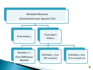
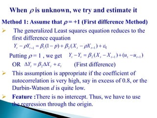
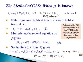
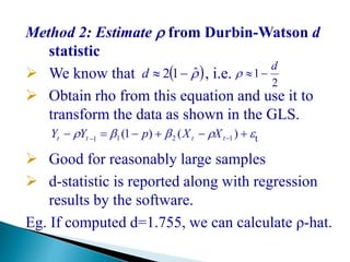
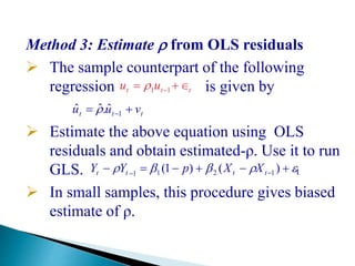
This document discusses remedies for autocorrelation in regression analysis. There are three main methods: 1. Assume ρ=1 and use first differencing to remove the autocorrelation. 2. Estimate ρ from the Durbin-Watson statistic and use it to transform the data in the generalized least squares (GLS) model. 3. Estimate ρ from the OLS residuals and use it to run GLS, though this may be biased in small samples. 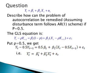The document also provides an example of applying GLS if the autocorrelation coefficient ρ is estimated to be 0.5.

1. Autocorrelation -
Remedies
Shilpa Chaudhary
JDMC

2. Remedial Measures
(Generalized Least Squares GLS)
If we know ρ
If we don’t
know ρ
Assume ρ=1
First Difference
Method
Estimate ρ from
DW d-statistic
Estimate ρ from
OLS residuals (et)

3.  If the regression holds at time t, it should hold at
time t-1, i.e.
 (2)
 Multiplying the second equation by
 gives
(3)
 Subtracting (3) from (1) gives
t
11211   ttt uXY 
11211 
 ttt uXY 
  
)()1( 1211 tttt XXpYY
ttt uXY  21  11  
AR(1) scheme
Follows all CLRM
assumptions. So
the TRICK is to
REPLACE ut with
this term in the
regression
(1)

4.  The equation can be re-written as:
 The error term satisfies all the OLS assumptions
 When we apply OLS to transformed models, the
estimators thus obtained are called generalized least
squares (GLS) estimators
 The estimators thus obtained will have the desirable
BLUE property

5.  Note that when we use GLS, we loose the first
observation. Eg. If n=50, now the GLS regression
will be run for 49 observations.
t
 To avoid this loss of one observation, the first
observation of Y and X is transformed as follows:
 Not generally used in large samples
 In small samples, results may be sensitive if we
exclude first observation.
  
)()1( 1211 tttt XXpYY

6. Method 1: Assume that  = +1 (First difference Method)
 The generalized Least squares equation reduces to the
first difference equation
t
Putting  = 1 , we get
OR (First difference)
 This assumption is appropriate if the coefficient of
autocorrelation is very high, say in excess of 0.8, or the
Durbin-Watson d is quite low.
 Feature :There is no intercept. Thus, we have to use
the regression through the origin.
)()( 112   tttttt uuXXYY 
ttt XY   2
  
)()1( 1211 tttt XXpYY

7. Method 2: Estimate  from Durbin-Watson d
statistic
 We know that , i.e.
 Obtain rho from this equation and use it to
transform the data as shown in the GLS.
t
 Good for reasonably large samples
 d-statistic is reported along with regression
results by the software.
Eg. If computed d=1.755, we can calculate ρ-hat.
2
1
d
 ˆ12 d
  
)()1( 1211 tttt XXpYY

8. Method 3: Estimate  from OLS residuals
 The sample counterpart of the following
regression is given by
 Estimate the above equation using OLS
residuals and obtain estimated-ρ. Use it to run
GLS. t
 In small samples, this procedure gives biased
estimate of ρ.
ttt uu  11
ttt vuu  1
ˆ.ˆˆ 
  
)()1( 1211 tttt XXpYY

9. Describe how can the problem of
autocorrelation be remedied (Assuming
disturbance term follows AR(1) scheme) if
P=0.5.
The GLS equation is:
t
Put ρ=0.5, we get
i.e.
ttt uXY  21 
  
)()1( 1211 tttt XXpYY

10. Thank you