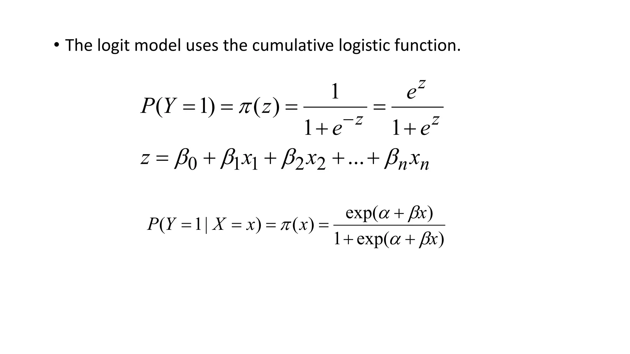
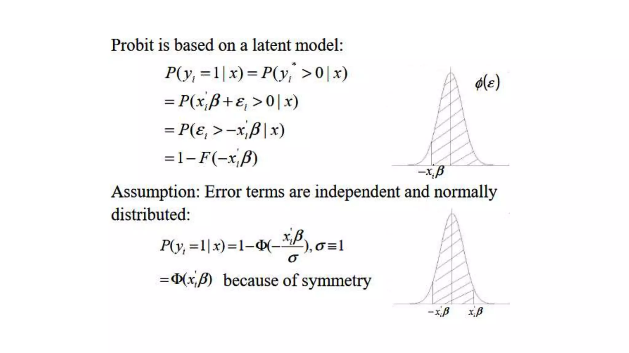
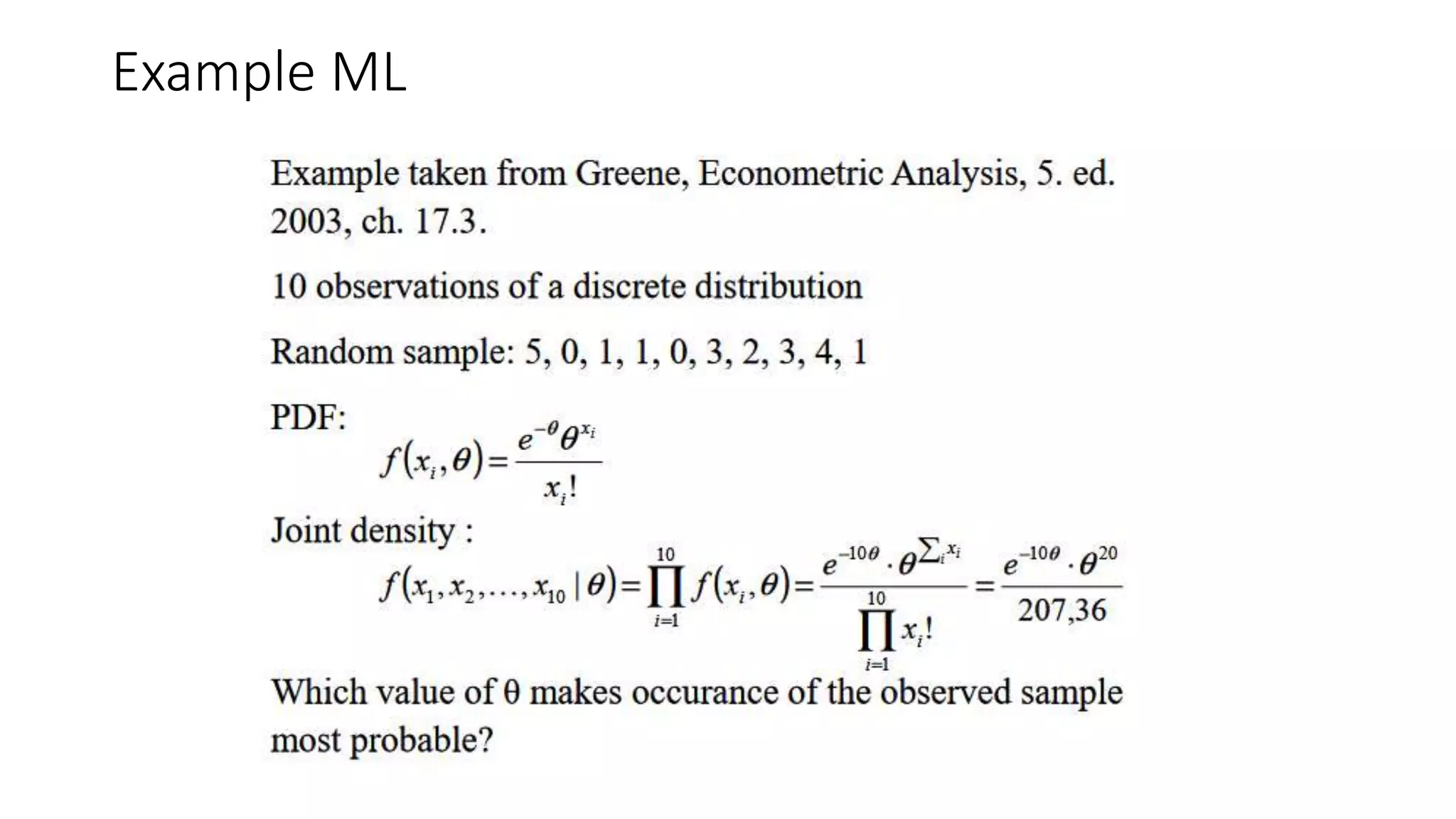
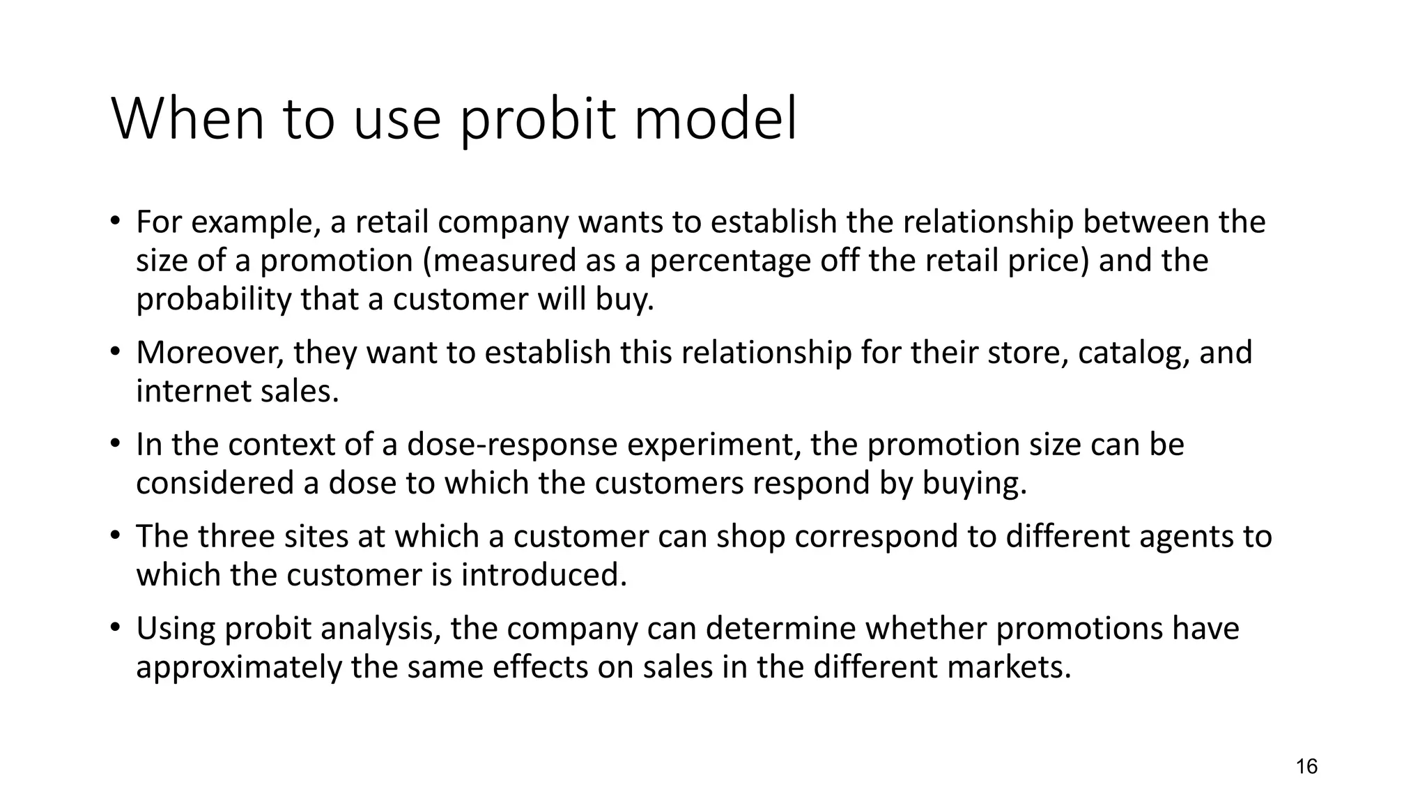
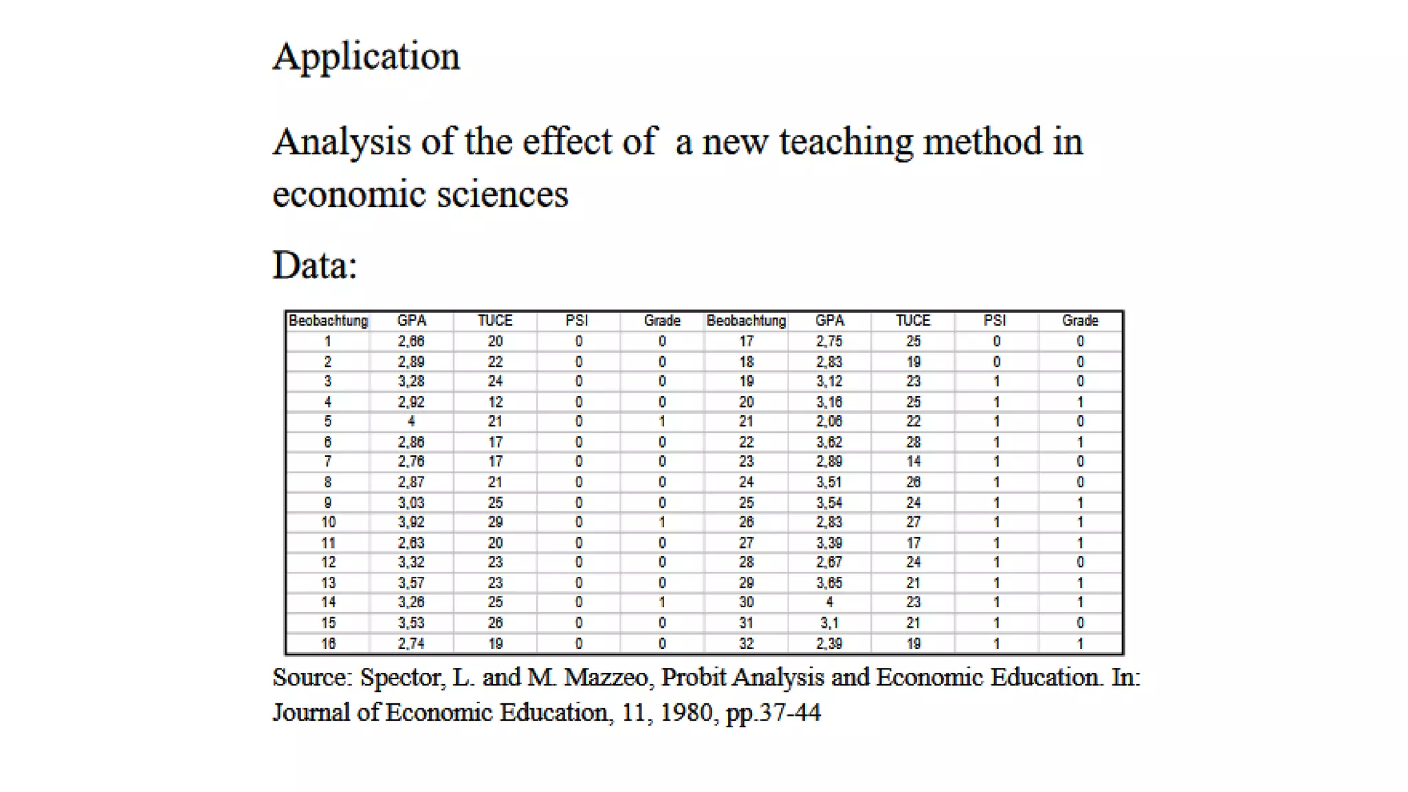
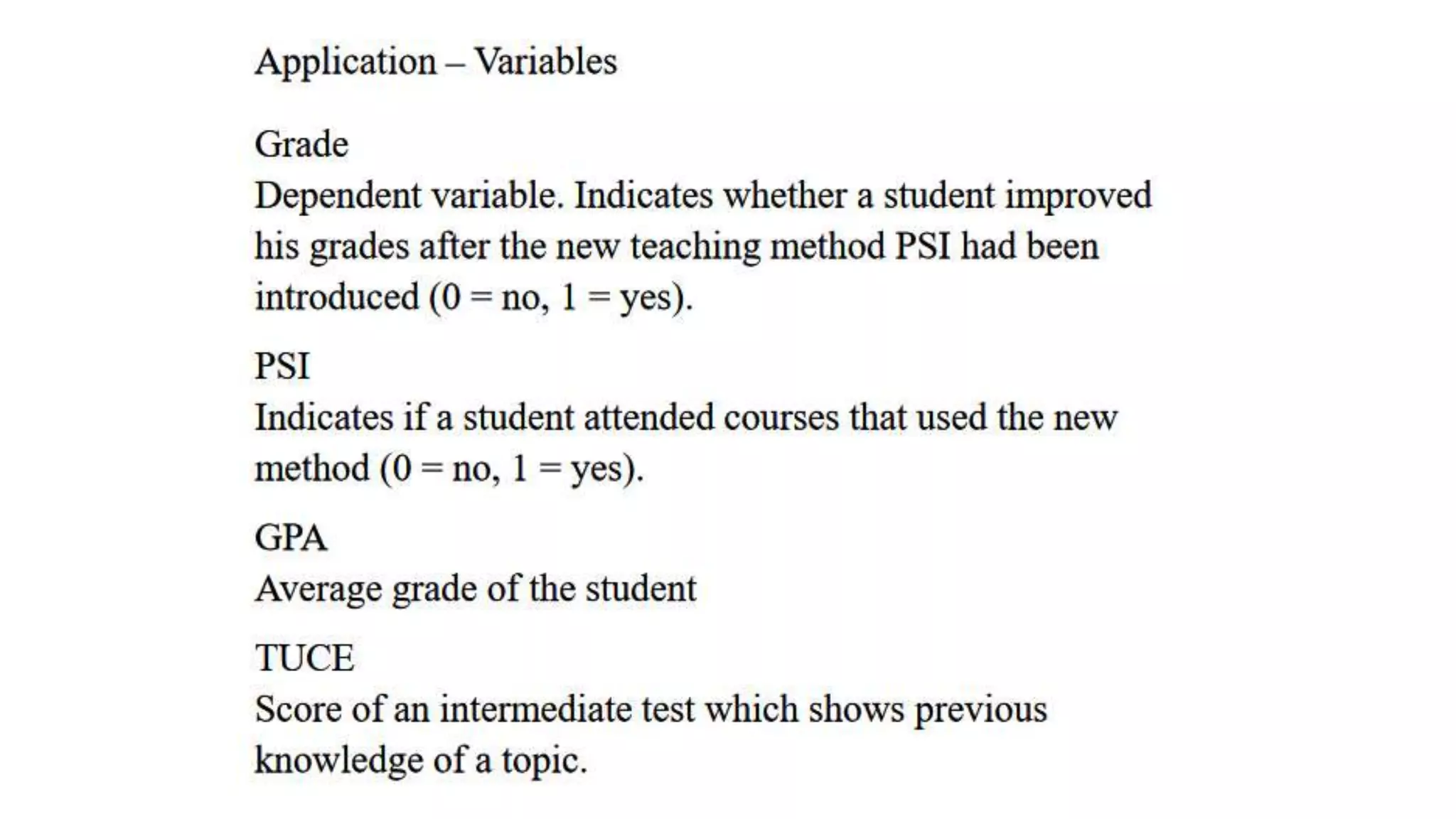
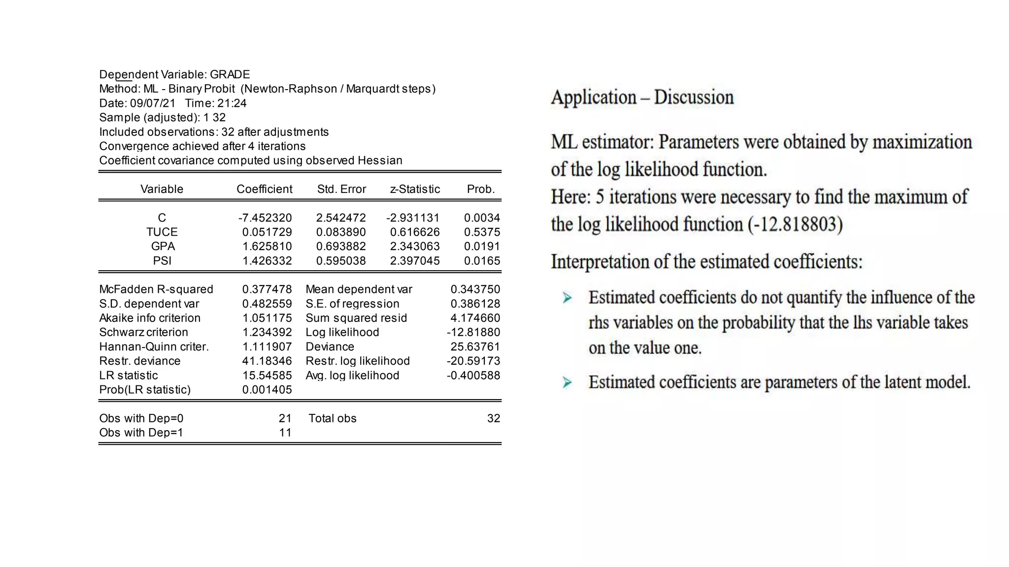
The probit model is appropriate when estimating the effects of independent variables on a binomial dependent variable from a dose-response experiment. It uses the normal cumulative distribution function. The document provides an example of using a probit model to analyze the relationship between promotion size (dose) and customer purchase probability (response) across different retail channels. It also gives an example application using probit analysis to estimate the effects of GPA, entrance exam score, and teaching method on student final grade.

1. The Probit Model

2. • The logit model uses the cumulative logistic function.
n
n
z
z
z
x
x
x
z
e
e
e
z
Y
P

















...
1
1
1
)
(
)
1
(
2
2
1
1
0
)
exp(
1
)
exp(
)
(
)
|
1
(
x
x
x
x
X
Y
P













3. • In some applications, the Normal CDF has been found useful.
• The estimating model that emerges from the Normal CDF is popularly
known as the probit model. Although sometimes it is also known as
the Normit model.
• In principle one could substitute the Normal CDF in place of logistic
CDF

9. The ML principle

10. The ML principle

11. Example ML

16. When to use probit model
• For example, a retail company wants to establish the relationship between the
size of a promotion (measured as a percentage off the retail price) and the
probability that a customer will buy.
• Moreover, they want to establish this relationship for their store, catalog, and
internet sales.
• In the context of a dose-response experiment, the promotion size can be
considered a dose to which the customers respond by buying.
• The three sites at which a customer can shop correspond to different agents to
which the customer is introduced.
• Using probit analysis, the company can determine whether promotions have
approximately the same effects on sales in the different markets.
16

17. 17
Grade = 1, if the final grade is A;
= 0, if the final grade is B or C
Explanatory variables are
• Grade Point Average (GPA),
• TUCE (Score on an examination given at the beginning of the term to test
entering knowledge of macroeconomics)
• Personalized System of Instruction (PSI);
PSI = 1, if new teaching method is used
= 0, otherwise
Application on Probit model

18. • Probit analysis is most appropriate when we would like to
estimate the effects of one or more independent variables on a
binomial dependent variable, particularly in the setting of a
dose-response experiment.
18

21. Dependent Variable: GRADE
Method: ML - Binary Probit (Newton-Raphson / Marquardt steps)
Date: 09/07/21 Time: 21:24
Sample (adjusted): 1 32
Included observations: 32 after adjustments
Convergence achieved after 4 iterations
Coefficient covariance computed using observed Hessian
Variable Coefficient Std. Error z-Statistic Prob.
C -7.452320 2.542472 -2.931131 0.0034
TUCE 0.051729 0.083890 0.616626 0.5375
GPA 1.625810 0.693882 2.343063 0.0191
PSI 1.426332 0.595038 2.397045 0.0165
McFadden R-squared 0.377478 Mean dependent var 0.343750
S.D. dependent var 0.482559 S.E. of regression 0.386128
Akaike info criterion 1.051175 Sum squared resid 4.174660
Schwarz criterion 1.234392 Log likelihood -12.81880
Hannan-Quinn criter. 1.111907 Deviance 25.63761
Restr. deviance 41.18346 Restr. log likelihood -20.59173
LR statistic 15.54585 Avg. log likelihood -0.400588
Prob(LR statistic) 0.001405
Obs with Dep=0 21 Total obs 32
Obs with Dep=1 11