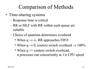
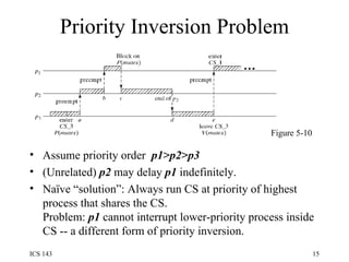
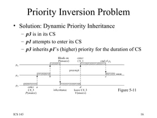
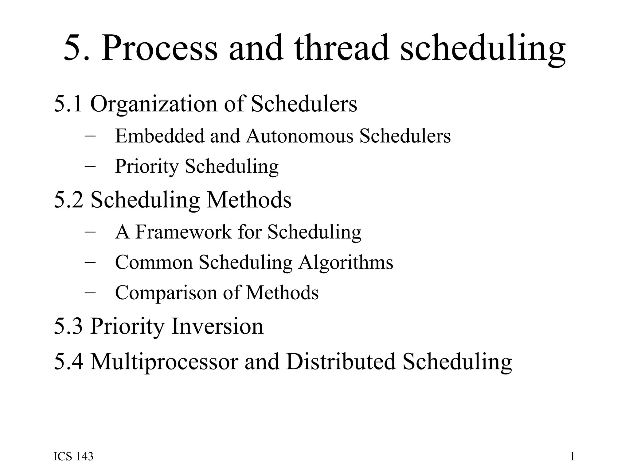
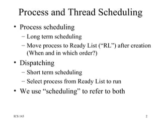
5. Process and thread scheduling 5.1 Organization of Schedulers  Embedded and Autonomous Schedulers  Priority Scheduling  5.2 Scheduling Methods  A Framework for Scheduling  Common Scheduling Algorithms  Comparison of Methods  5.3 Priority Inversion  5.4 Multiprocessor and Distributed Scheduling
Process and Thread Scheduling Process scheduling Long term scheduling Move process to Ready List (“RL”) after creation (When and in which order?) Dispatching Short term scheduling Select process from Ready List to run We use “scheduling” to refer to both
Organization of Schedulers Embedded Called as function at end of kernel call Runs as part of calling process Autonomous Separate process May have dedicated CPU on a multiprocessor On single-processor, run at every quantum: scheduler and other processes alternate Figure 5-1
Priority Scheduling Priority function returns numerical value  P  for process  p :  P = Priority(p) Static priority: unchanged for lifetime of  p Dynamic priority: changes at runtime Priority divides processes into levels implemented as multi-level RL p  at RL[ i ] run before  q  at RL[ j ] if  i>j p, q  at same level are ordered by other criteria
An Embedded Scheduler Scheduler() {  do {  Find highest priority  ready_a  process p;  Find a free cpu;  if (cpu != NIL) Allocate_CPU(p,cpu);  } while (cpu != NIL);  do {  Find highest priority  ready_a  process p;  Find lowest priority  running  process q;  if (Priority(p) > Priority(q)) Preempt(p,q);  } while (Priority(p) > Priority(q)); if (self->Status.Type!=’running’) Preempt(p,self);  }
Scheduling Methods When is scheduler invoked? Decision mode Preemptive: scheduler called periodically (quantum-oriented) or when system state changes Nonpreemptive: scheduler called when process terminates or blocks How does it select highest priority process? Priority function:  P = Priority(p) Arbitration rule: break ties  Random Chronological (First In First Out = FIFO) Cyclic (Round Robin = RR)
Priority function Possible parameters: Attained service time ( a ) Real time in system ( r ) Total service time ( t ) Period ( d ) Deadline (explicit or implied by period) External priority ( e ) Memory requirements (mostly for batch) System load (not process-specific)
Scheduling algorithms Name, Decision mode, Priority,  Arbitration FIFO:  nonpreemptive  P = r     random SJF:  nonpreemptive  P = –t     chronolgcl/random SRT:  preemptive  P = –(t–a)  chronolgcl/random RR:  preemptive  P = 0     cyclic ML:  preemptive    P = e     cyclic nonpreemptive  P = e     chronological n fixed priority levels level P is serviced when n  through P+1 empty
MLF (Multilevel Feedback) Like ML, but priority changes dynamically E very process enters at highest level  n Each level P prescribes maximum time  t P t P  increases as P decreases Typically:  t n  = T  (constant) t P   = 2    t P+1   Figure 5-3
Scheduling algorithms MLF priority function:  Find  P = n–i  for given  a :   priority  attained time n a<T n–1  a<T+2T n–2  a<T+2T+4T . . .  . . . n–i  a<(2 i+1 –1)T Find smallest  i  such that  a<(2 i+1 –1)T : Solve for  i :  i =   lg 2 (a/T+1)   P = n–i = n–   lg 2 (a/T+1) 
Scheduling Algorithms Rate Monotonic (RM):  Intended for periodic (real-time) processes Preemptive  Highest priority: shortest period:  P = –d Earliest Deadline First (EDF): Intended for periodic (real-time) processes Preemptive  Highest priority: shortest time to next deadline r    d     number of completed periods r % d     time in current period d – r % d     time remaining in current period P = –(d – r % d)
Comparison of Methods FIFO, SJF, SRT: Primarily for batch systems FIFO simplest, SJF & SRT have better average turnaround times:  (r1+r2+…+rn)/n FIFO: ((0+5) + (3+2))/2 = 5.0 SRT:  ((2+5) + (0+2))/2 = 4.5 Figure 5-2
Comparison of Methods Time-sharing systems Response time is critical RR or MLF with RR within each queue are suitable Choice of quantum determines overhead When q      , RR approaches FIFO When q    0, context switch overhead    100% When q >> context switch overhead, n processes run concurrently at 1/n CPU speed
Comparison of Methods Real-time systems Feasible = All deadlines are met CPU utilization is defined as: U= ∑ t i /d i Schedule is feasible if U    1 EDF always yields feasible schedule (if U    1) RM yields feasible schedule if U    0.7 Figure 5-9
Priority Inversion Problem Assume priority order  p1>p2>p3 (Unrelated)  p2  may delay  p1  indefinitely. Naïve “solution”: Always run CS at priority of highest process that shares the CS. Problem:  p1  cannot interrupt lower-priority process inside CS -- a different form of priority inversion. Figure 5-10
Priority Inversion Problem Solution: Dynamic Priority Inheritance p3  is in its CS p1  attempts to enter its CS p3  inherits  p1 ’s (higher) priority for the duration of CS Figure 5-11

Os5

  • 1.
    5. Process andthread scheduling 5.1 Organization of Schedulers Embedded and Autonomous Schedulers Priority Scheduling 5.2 Scheduling Methods A Framework for Scheduling Common Scheduling Algorithms Comparison of Methods 5.3 Priority Inversion 5.4 Multiprocessor and Distributed Scheduling
  • 2.
    Process and ThreadScheduling Process scheduling Long term scheduling Move process to Ready List (“RL”) after creation (When and in which order?) Dispatching Short term scheduling Select process from Ready List to run We use “scheduling” to refer to both
  • 3.
    Organization of SchedulersEmbedded Called as function at end of kernel call Runs as part of calling process Autonomous Separate process May have dedicated CPU on a multiprocessor On single-processor, run at every quantum: scheduler and other processes alternate Figure 5-1
  • 4.
    Priority Scheduling Priorityfunction returns numerical value P for process p : P = Priority(p) Static priority: unchanged for lifetime of p Dynamic priority: changes at runtime Priority divides processes into levels implemented as multi-level RL p at RL[ i ] run before q at RL[ j ] if i>j p, q at same level are ordered by other criteria
  • 5.
    An Embedded SchedulerScheduler() { do { Find highest priority ready_a process p; Find a free cpu; if (cpu != NIL) Allocate_CPU(p,cpu); } while (cpu != NIL); do { Find highest priority ready_a process p; Find lowest priority running process q; if (Priority(p) > Priority(q)) Preempt(p,q); } while (Priority(p) > Priority(q)); if (self->Status.Type!=’running’) Preempt(p,self); }
  • 6.
    Scheduling Methods Whenis scheduler invoked? Decision mode Preemptive: scheduler called periodically (quantum-oriented) or when system state changes Nonpreemptive: scheduler called when process terminates or blocks How does it select highest priority process? Priority function: P = Priority(p) Arbitration rule: break ties Random Chronological (First In First Out = FIFO) Cyclic (Round Robin = RR)
  • 7.
    Priority function Possibleparameters: Attained service time ( a ) Real time in system ( r ) Total service time ( t ) Period ( d ) Deadline (explicit or implied by period) External priority ( e ) Memory requirements (mostly for batch) System load (not process-specific)
  • 8.
    Scheduling algorithms Name,Decision mode, Priority, Arbitration FIFO: nonpreemptive P = r random SJF: nonpreemptive P = –t chronolgcl/random SRT: preemptive P = –(t–a) chronolgcl/random RR: preemptive P = 0 cyclic ML: preemptive P = e cyclic nonpreemptive P = e chronological n fixed priority levels level P is serviced when n through P+1 empty
  • 9.
    MLF (Multilevel Feedback)Like ML, but priority changes dynamically E very process enters at highest level n Each level P prescribes maximum time t P t P increases as P decreases Typically: t n = T (constant) t P = 2  t P+1 Figure 5-3
  • 10.
    Scheduling algorithms MLFpriority function: Find P = n–i for given a : priority attained time n a<T n–1 a<T+2T n–2 a<T+2T+4T . . . . . . n–i a<(2 i+1 –1)T Find smallest i such that a<(2 i+1 –1)T : Solve for i : i =  lg 2 (a/T+1)  P = n–i = n–  lg 2 (a/T+1) 
  • 11.
    Scheduling Algorithms RateMonotonic (RM): Intended for periodic (real-time) processes Preemptive Highest priority: shortest period: P = –d Earliest Deadline First (EDF): Intended for periodic (real-time) processes Preemptive Highest priority: shortest time to next deadline r  d number of completed periods r % d time in current period d – r % d time remaining in current period P = –(d – r % d)
  • 12.
    Comparison of MethodsFIFO, SJF, SRT: Primarily for batch systems FIFO simplest, SJF & SRT have better average turnaround times: (r1+r2+…+rn)/n FIFO: ((0+5) + (3+2))/2 = 5.0 SRT: ((2+5) + (0+2))/2 = 4.5 Figure 5-2
  • 13.
    Comparison of MethodsTime-sharing systems Response time is critical RR or MLF with RR within each queue are suitable Choice of quantum determines overhead When q   , RR approaches FIFO When q  0, context switch overhead  100% When q >> context switch overhead, n processes run concurrently at 1/n CPU speed
  • 14.
    Comparison of MethodsReal-time systems Feasible = All deadlines are met CPU utilization is defined as: U= ∑ t i /d i Schedule is feasible if U  1 EDF always yields feasible schedule (if U  1) RM yields feasible schedule if U  0.7 Figure 5-9
  • 15.
    Priority Inversion ProblemAssume priority order p1>p2>p3 (Unrelated) p2 may delay p1 indefinitely. Naïve “solution”: Always run CS at priority of highest process that shares the CS. Problem: p1 cannot interrupt lower-priority process inside CS -- a different form of priority inversion. Figure 5-10
  • 16.
    Priority Inversion ProblemSolution: Dynamic Priority Inheritance p3 is in its CS p1 attempts to enter its CS p3 inherits p1 ’s (higher) priority for the duration of CS Figure 5-11