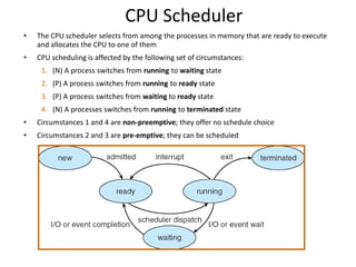
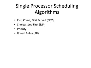
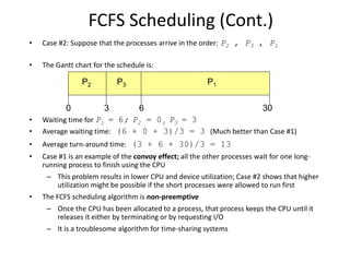
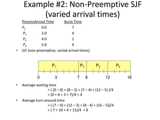
This document discusses CPU scheduling algorithms. It begins with basic concepts like multiprogramming and the alternating cycle of CPU and I/O bursts that processes undergo. It then covers key scheduling criteria like CPU utilization, throughput, waiting time and turnaround time. Several single processor scheduling algorithms are explained in detail, including first come first served (FCFS), shortest job first (SJF), priority scheduling, and round robin (RR). Examples are provided to illustrate how each algorithm works. Finally, it briefly introduces the concept of multi-level queue scheduling using multiple queues to classify different types of processes.

1. CPU Scheduling (Algorithms)
Lecture 11,12
by Mr MOHAMMAD NAZIR

2. Agenda
• 5.1 Basic Concepts
• 5.2 Scheduling Criteria
• 5.3 Scheduling Algorithms
• 5.4 Multiple-Processor Scheduling
• 5.5 Thread Scheduling (skip)
• 5.6 Operating System Examples
• 5.7 Algorithm Evaluation

3. 5.1 Basic Concepts

4. Basic Concepts
• Maximum CPU utilization is obtained with multiprogramming
– Several processes are kept in memory at one time
– Every time a running process has to wait, another process can take
over use of the CPU
• Scheduling of the CPU is fundamental to operating system design
• Process execution consists of a cycle of a CPU time burst and an I/O time
burst (i.e. wait) as shown on the next slide
– Processes alternate between these two states (i.e., CPU burst and I/O
burst)
– Eventually, the final CPU burst ends with a system request to terminate
execution

5. Alternating Sequence of CPU And I/O Bursts

6. Histogram of CPU-burst Times
CPU bursts tend to have a frequency curve similar to the exponential curve shown
above. It is characterized by a large number of short CPU bursts and a small number of
long CPU bursts. An I/O-bound program typically has many short CPU bursts; a CPU-
bound program might have a few long CPU bursts.

7. CPU Scheduler
• The CPU scheduler selects from among the processes in memory that are ready to execute
and allocates the CPU to one of them
• CPU scheduling is affected by the following set of circumstances:
1. (N) A process switches from running to waiting state
2. (P) A process switches from running to ready state
3. (P) A process switches from waiting to ready state
4. (N) A processes switches from running to terminated state
• Circumstances 1 and 4 are non-preemptive; they offer no schedule choice
• Circumstances 2 and 3 are pre-emptive; they can be scheduled

8. Dispatcher
• The dispatcher module gives control of the CPU to the process selected by the
short-term scheduler; this involves:
– switching context
– switching to user mode
– jumping to the proper location in the user program to restart that program
• The dispatcher needs to run as fast as possible, since it is invoked during process
context switch
• The time it takes for the dispatcher to stop one process and start another process
is called dispatch latency

9. 5.2 Scheduling Criteria

10. Scheduling Criteria
• Different CPU scheduling algorithms have different properties
• The choice of a particular algorithm may favor one class of processes over another
• In choosing which algorithm to use, the properties of the various algorithms should be
considered
• Criteria for comparing CPU scheduling algorithms may include the following
– CPU utilization – percent of time that the CPU is busy executing a process
– Throughput – number of processes that are completed per time unit
– Response time – amount of time it takes from when a request was submitted until the
first response occurs (but not the time it takes to output the entire response)
– Waiting time – the amount of time before a process starts after first entering the
ready queue (or the sum of the amount of time a process has spent waiting in the
ready queue)
– Turnaround time – amount of time to execute a particular process from the time of
submission through the time of completion

11. Optimization Criteria
• It is desirable to
– Maximize CPU utilization
– Maximize throughput
– Minimize turnaround time
– Minimize start time
– Minimize waiting time
– Minimize response time
• In most cases, we strive to optimize the average measure of each metric
• In other cases, it is more important to optimize the minimum or maximum values
rather than the average

12. 5.3a Single Processor Scheduling
Algorithms

13. Single Processor Scheduling
Algorithms
• First Come, First Served (FCFS)
• Shortest Job First (SJF)
• Priority
• Round Robin (RR)

14. First Come, First Served (FCFS)
Scheduling

15. First-Come, First-Served (FCFS) Scheduling
Process Burst Time
P1 24
P2 3
P3 3
• With FCFS, the process that requests the CPU first is allocated the CPU first
• Case #1: Suppose that the processes arrive in the order: P1 , P2 , P3
The Gantt Chart for the schedule is:
• Waiting time for P1 = 0; P2 = 24; P3 = 27
• Average waiting time: (0 + 24 + 27)/3 = 17
• Average turn-around time: (24 + 27 + 30)/3 = 27
P1 P2 P3
24 27 300

16. FCFS Scheduling (Cont.)
• Case #2: Suppose that the processes arrive in the order: P2 , P3 , P1
• The Gantt chart for the schedule is:
• Waiting time for P1 = 6; P2 = 0; P3 = 3
• Average waiting time: (6 + 0 + 3)/3 = 3 (Much better than Case #1)
• Average turn-around time: (3 + 6 + 30)/3 = 13
• Case #1 is an example of the convoy effect; all the other processes wait for one long-
running process to finish using the CPU
– This problem results in lower CPU and device utilization; Case #2 shows that higher
utilization might be possible if the short processes were allowed to run first
• The FCFS scheduling algorithm is non-preemptive
– Once the CPU has been allocated to a process, that process keeps the CPU until it
releases it either by terminating or by requesting I/O
– It is a troublesome algorithm for time-sharing systems
P1P3P2
63 300

17. Shortest Job First (SJF) Scheduling

18. Shortest-Job-First (SJF) Scheduling
• The SJF algorithm associates with each process the length of its next CPU burst
• When the CPU becomes available, it is assigned to the process that has the
smallest next CPU burst (in the case of matching bursts, FCFS is used)
• Two schemes:
– Nonpreemptive – once the CPU is given to the process, it cannot be
preempted until it completes its CPU burst
– Preemptive – if a new process arrives with a CPU burst length less than the
remaining time of the current executing process, preempt. This scheme is
know as the Shortest-Remaining-Time-First (SRTF)

19. Example #1: Non-Preemptive SJF
(simultaneous arrival)
ProcessArrival Time Burst Time
P1 0.0 6
P2 0.0 4
P3 0.0 1
P4 0.0 5
• SJF (non-preemptive, simultaneous arrival)
• Average waiting time = (0 + 1 + 5 + 10)/4 = 4
• Average turn-around time = (1 + 5 + 10 + 16)/4 = 8
P1P3 P2
51 160
P4
10

20. Example #2: Non-Preemptive SJF
(varied arrival times)
ProcessArrival Time Burst Time
P1 0.0 7
P2 2.0 4
P3 4.0 1
P4 5.0 4
• SJF (non-preemptive, varied arrival times)
• Average waiting time
= ( (0 – 0) + (8 – 2) + (7 – 4) + (12 – 5) )/4
= (0 + 6 + 3 + 7)/4 = 4
• Average turn-around time:
= ( (7 – 0) + (12 – 2) + (8 - 4) + (16 – 5))/4
= ( 7 + 10 + 4 + 11)/4 = 8
P1 P3 P2
73 160
P4
8 12

21. Example #3: Preemptive SJF
(Shortest-remaining-time-first)
ProcessArrival Time Burst Time
P1 0.0 7
P2 2.0 4
P3 4.0 1
P4 5.0 4
• SJF (pre-emptive, varied arrival times)
• Average waiting time
= ( [(0 – 0) + (11 - 2)] + [(2 – 2) + (5 – 4)] + (4 - 4) + (7 – 5) )/4
= 9 + 1 + 0 + 2)/4
= 3
• Average turn-around time = (16 + 7 + 5 + 11)/4 = 9.75
P1 P3P2
42 110
P4
5 7
P2 P1
16
Waiting time : sum of time that a process has spent waiting in the ready queue

22. Priority Scheduling

23. Priority Scheduling
• The SJF algorithm is a special case of the general priority scheduling algorithm
• A priority number (integer) is associated with each process
• The CPU is allocated to the process with the highest priority (smallest integer =
highest priority)
• Priority scheduling can be either preemptive or non-preemptive
– A preemptive approach will preempt the CPU if the priority of the newly-
arrived process is higher than the priority of the currently running process
– A non-preemptive approach will simply put the new process (with the highest
priority) at the head of the ready queue
• SJF is a priority scheduling algorithm where priority is the predicted next CPU burst
time
• The main problem with priority scheduling is starvation, that is, low priority
processes may never execute
• A solution is aging; as time progresses, the priority of a process in the ready queue
is increased

24. Round Robin (RR) Scheduling

25. Round Robin (RR) Scheduling
• In the round robin algorithm, each process gets a small unit of CPU time (a time
quantum), usually 10-100 milliseconds. After this time has elapsed, the process is
preempted and added to the end of the ready queue.
• If there are n processes in the ready queue and the time quantum is q, then each
process gets 1/n of the CPU time in chunks of at most q time units at once. No process
waits more than (n-1)q time units.
• Performance of the round robin algorithm
– q large  FCFS
– q small  q must be greater than the context switch time; otherwise, the
overhead is too high
• One rule of thumb is that 80% of the CPU bursts should be shorter than the time
quantum

26. Example of RR with Time Quantum =
20
Process Burst Time
P1 53
P2 17
P3 68
P4 24
• The Gantt chart is:
• Typically, higher average turnaround than SJF, but better response time
• Average waiting time
= ( [(0 – 0) + (77 - 20) + (121 – 97)] + (20 – 0) + [(37 – 0) + (97 - 57) + (134 – 117)] + [(57
– 0) + (117 – 77)] ) / 4
= (0 + 57 + 24) + 20 + (37 + 40 + 17) + (57 + 40) ) / 4
= (81 + 20 + 94 + 97)/4
= 292 / 4 = 73
• Average turn-around time = 134 + 37 + 162 + 121) / 4 = 113.5
P1 P2 P3 P4 P1 P3 P4 P1 P3 P3
0 20 37 57 77 97 117 121 134 154 162

27. Time Quantum and Context Switches

28. Turnaround Time Varies With The Time Quantum
As can be seen from this graph, the average turnaround time of a set
of processes does not necessarily improve as the time quantum size
increases. In general, the average turnaround time can be improved
if most processes finish their next CPU burst in a single time quantum.

29. 5.3b Multi-level Queue Scheduling

30. Multi-level Queue Scheduling
• Multi-level queue scheduling is used when processes can be classified into groups
• For example, foreground (interactive) processes and background (batch) processes
– The two types of processes have different response-time requirements and so may have
different scheduling needs
– Also, foreground processes may have priority (externally defined) over background
processes
• A multi-level queue scheduling algorithm partitions the ready queue into several separate
queues
• The processes are permanently assigned to one queue, generally based on some property of
the process such as memory size, process priority, or process type
• Each queue has its own scheduling algorithm
– The foreground queue might be scheduled using an RR algorithm
– The background queue might be scheduled using an FCFS algorithm
• In addition, there needs to be scheduling among the queues, which is commonly implemented
as fixed-priority pre-emptive scheduling
– The foreground queue may have absolute priority over the background queue

31. Multi-level Queue Scheduling
• One example of a multi-level queue are the five queues shown below
• Each queue has absolute priority over lower priority queues
• For example, no process in the batch queue can run unless the queues above it are
empty
• However, this can result in starvation for the processes in the lower priority queues

32. Multilevel Queue Scheduling
• Another possibility is to time slice among the queues
• Each queue gets a certain portion of the CPU time, which it can then schedule
among its various processes
– The foreground queue can be given 80% of the CPU time for RR scheduling
– The background queue can be given 20% of the CPU time for FCFS scheduling

33. 5.3c Multi-level Feedback Queue
Scheduling

34. Multilevel Feedback Queue
Scheduling
• In multi-level feedback queue scheduling, a process can move between the various
queues; aging can be implemented this way
• A multilevel-feedback-queue scheduler is defined by the following parameters:
– Number of queues
– Scheduling algorithms for each queue
– Method used to determine when to promote a process
– Method used to determine when to demote a process
– Method used to determine which queue a process will enter when that
process needs service

35. Example of Multilevel Feedback
Queue
• Scheduling
– A new job enters queue Q0 (RR) and is placed at the end. When it gains the
CPU, the job receives 8 milliseconds. If it does not finish in 8 milliseconds, the
job is moved to the end of queue Q1.
– A Q1 (RR) job receives 16 milliseconds. If it still does not complete, it is
preempted and moved to queue Q2 (FCFS).
Q0
Q1
Q2