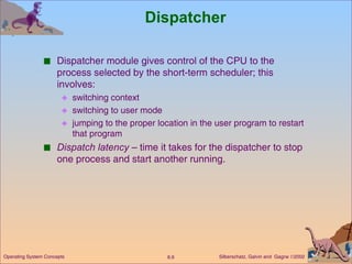
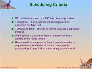
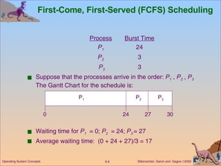
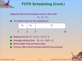
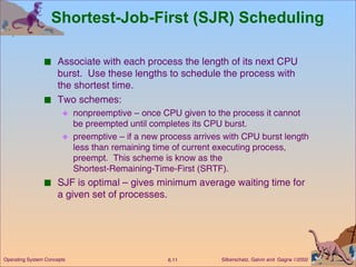
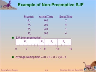
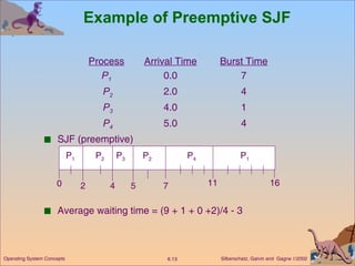
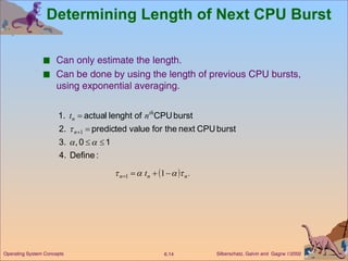
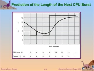
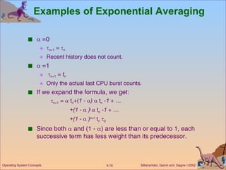
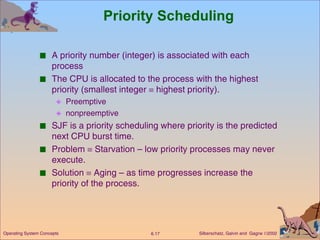
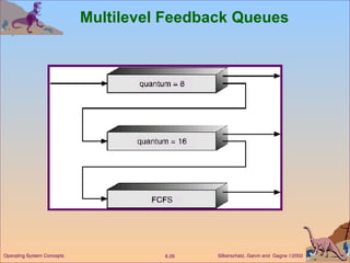
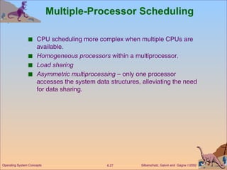
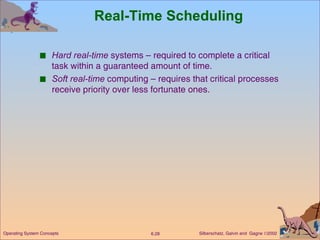
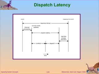
This document discusses various CPU scheduling algorithms and concepts. It covers scheduling criteria like CPU utilization and turnaround time. Algorithms discussed include first-come first-served (FCFS), shortest job first (SJF), priority scheduling, and round robin (RR). It also covers multiple processor scheduling, real-time scheduling, and evaluating scheduling algorithms.

1. Chapter 6: CPU Scheduling Basic Concepts Scheduling Criteria Scheduling Algorithms Multiple-Processor Scheduling Real-Time Scheduling Algorithm Evaluation

2. Basic Concepts Maximum CPU utilization obtained with multiprogramming CPU–I/O Burst Cycle – Process execution consists of a cycle of CPU execution and I/O wait. CPU burst distribution

3. Alternating Sequence of CPU And I/O Bursts

4. Histogram of CPU-burst Times

5. CPU Scheduler Selects from among the processes in memory that are ready to execute, and allocates the CPU to one of them. CPU scheduling decisions may take place when a process: 1. Switches from running to waiting state. 2. Switches from running to ready state. 3. Switches from waiting to ready. 4. Terminates. Scheduling under 1 and 4 is nonpreemptive . All other scheduling is preemptive.

6. Dispatcher Dispatcher module gives control of the CPU to the process selected by the short-term scheduler; this involves: switching context switching to user mode jumping to the proper location in the user program to restart that program Dispatch latency – time it takes for the dispatcher to stop one process and start another running.

7. Scheduling Criteria CPU utilization – keep the CPU as busy as possible Throughput – # of processes that complete their execution per time unit Turnaround time – amount of time to execute a particular process Waiting time – amount of time a process has been waiting in the ready queue Response time – amount of time it takes from when a request was submitted until the first response is produced, not output (for time-sharing environment)

8. Optimization Criteria Max CPU utilization Max throughput Min turnaround time Min waiting time Min response time

9. First-Come, First-Served (FCFS) Scheduling Process Burst Time P 1 24 P 2 3 P 3 3 Suppose that the processes arrive in the order: P 1 , P 2 , P 3 The Gantt Chart for the schedule is: Waiting time for P 1 = 0; P 2 = 24; P 3 = 27 Average waiting time: (0 + 24 + 27)/3 = 17 P 1 P 2 P 3 24 27 30 0

10. FCFS Scheduling (Cont.) Suppose that the processes arrive in the order P 2 , P 3 , P 1 . The Gantt chart for the schedule is: Waiting time for P 1 = 6 ; P 2 = 0 ; P 3 = 3 Average waiting time: (6 + 0 + 3)/3 = 3 Much better than previous case. Convoy effect short process behind long process P 1 P 3 P 2 6 3 30 0

11. Shortest-Job-First (SJR) Scheduling Associate with each process the length of its next CPU burst. Use these lengths to schedule the process with the shortest time. Two schemes: nonpreemptive – once CPU given to the process it cannot be preempted until completes its CPU burst. preemptive – if a new process arrives with CPU burst length less than remaining time of current executing process, preempt. This scheme is know as the Shortest-Remaining-Time-First (SRTF). SJF is optimal – gives minimum average waiting time for a given set of processes.

12. Process Arrival Time Burst Time P 1 0.0 7 P 2 2.0 4 P 3 4.0 1 P 4 5.0 4 SJF (non-preemptive) Average waiting time = (0 + 6 + 3 + 7)/4 - 4 Example of Non-Preemptive SJF P 1 P 3 P 2 7 3 16 0 P 4 8 12

13. Example of Preemptive SJF Process Arrival Time Burst Time P 1 0.0 7 P 2 2.0 4 P 3 4.0 1 P 4 5.0 4 SJF (preemptive) Average waiting time = (9 + 1 + 0 +2)/4 - 3 P 1 P 3 P 2 4 2 11 0 P 4 5 7 P 2 P 1 16

14. Determining Length of Next CPU Burst Can only estimate the length. Can be done by using the length of previous CPU bursts, using exponential averaging.

15. Prediction of the Length of the Next CPU Burst

16. Examples of Exponential Averaging  =0  n+1 =  n Recent history does not count.  =1  n+1 = t n Only the actual last CPU burst counts. If we expand the formula, we get:  n+1 =  t n +( 1 -  )  t n - 1 + … +(1 -  ) j  t n - 1 + … +(1 -  ) n=1 t n  0 Since both  and (1 -  ) are less than or equal to 1, each successive term has less weight than its predecessor.

17. Priority Scheduling A priority number (integer) is associated with each process The CPU is allocated to the process with the highest priority (smallest integer  highest priority). Preemptive nonpreemptive SJF is a priority scheduling where priority is the predicted next CPU burst time. Problem  Starvation – low priority processes may never execute. Solution  Aging – as time progresses increase the priority of the process.

18. Round Robin (RR) Each process gets a small unit of CPU time ( time quantum ), usually 10-100 milliseconds. After this time has elapsed, the process is preempted and added to the end of the ready queue. If there are n processes in the ready queue and the time quantum is q , then each process gets 1/ n of the CPU time in chunks of at most q time units at once. No process waits more than ( n -1) q time units. Performance q large  FIFO q small  q must be large with respect to context switch, otherwise overhead is too high.

19. Example of RR with Time Quantum = 20 Process Burst Time P 1 53 P 2 17 P 3 68 P 4 24 The Gantt chart is: Typically, higher average turnaround than SJF, but better response . P 1 P 2 P 3 P 4 P 1 P 3 P 4 P 1 P 3 P 3 0 20 37 57 77 97 117 121 134 154 162

20. Time Quantum and Context Switch Time

21. Turnaround Time Varies With The Time Quantum

22. Multilevel Queue Ready queue is partitioned into separate queues: foreground (interactive) background (batch) Each queue has its own scheduling algorithm, foreground – RR background – FCFS Scheduling must be done between the queues. Fixed priority scheduling; (i.e., serve all from foreground then from background). Possibility of starvation. Time slice – each queue gets a certain amount of CPU time which it can schedule amongst its processes; i.e., 80% to foreground in RR 20% to background in FCFS

23. Multilevel Queue Scheduling

24. Multilevel Feedback Queue A process can move between the various queues; aging can be implemented this way. Multilevel-feedback-queue scheduler defined by the following parameters: number of queues scheduling algorithms for each queue method used to determine when to upgrade a process method used to determine when to demote a process method used to determine which queue a process will enter when that process needs service

25. Example of Multilevel Feedback Queue Three queues: Q 0 – time quantum 8 milliseconds Q 1 – time quantum 16 milliseconds Q 2 – FCFS Scheduling A new job enters queue Q 0 which is served FCFS. When it gains CPU, job receives 8 milliseconds. If it does not finish in 8 milliseconds, job is moved to queue Q 1 . At Q 1 job is again served FCFS and receives 16 additional milliseconds. If it still does not complete, it is preempted and moved to queue Q 2 .

26. Multilevel Feedback Queues

27. Multiple-Processor Scheduling CPU scheduling more complex when multiple CPUs are available. Homogeneous processors within a multiprocessor. Load sharing Asymmetric multiprocessing – only one processor accesses the system data structures, alleviating the need for data sharing.

28. Real-Time Scheduling Hard real-time systems – required to complete a critical task within a guaranteed amount of time. Soft real-time computing – requires that critical processes receive priority over less fortunate ones.

29. Dispatch Latency

30. Algorithm Evaluation Deterministic modeling – takes a particular predetermined workload and defines the performance of each algorithm for that workload. Queueing models Implementation

31. Evaluation of CPU Schedulers by Simulation

32. Solaris 2 Scheduling

33. Windows 2000 Priorities