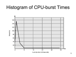
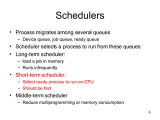
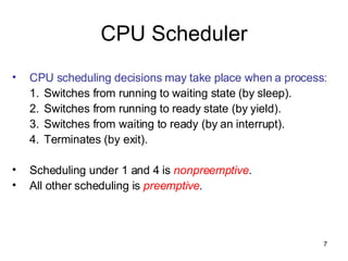
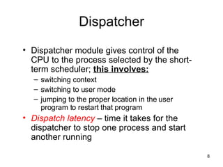
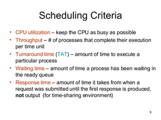
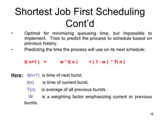
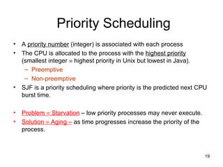
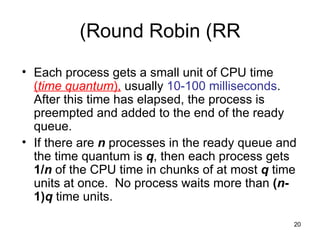
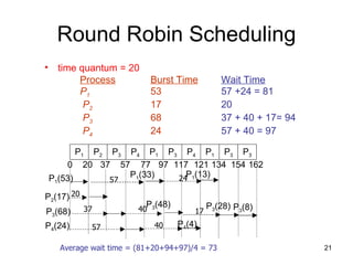
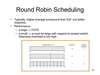
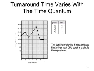
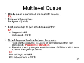
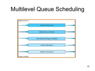
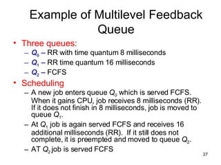
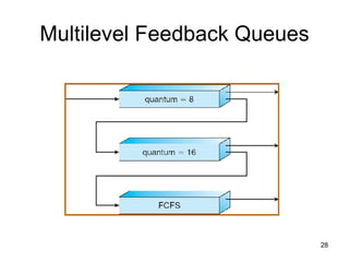
CPU Scheduling Chapter 5
CPU Scheduling Basic Concepts Scheduling Criteria  Scheduling Algorithms Multiple-Processor Scheduling Thread Scheduling UNIX example
Basic Concepts Maximum CPU utilization obtained with  multiprogramming CPU–I/O Burst Cycle  – Process execution consists of a  cycle  of CPU execution and I/O wait CPU times are generally much shorter than I/O times.
CPU-I/O Burst Cycle Process A Process B
Histogram of CPU-burst Times
Schedulers Process migrates among several queues Device queue, job queue, ready queue Scheduler selects a process to run from these queues Long-term scheduler:  load a job in memory Runs infrequently Short-term scheduler: Select ready process to run on CPU Should be fast Middle-term scheduler Reduce multiprogramming or memory consumption
CPU Scheduler CPU scheduling decisions may take place when a process: 1. Switches from running to waiting state (by sleep). 2. Switches from running to ready state (by yield). 3. Switches from waiting to ready (by an interrupt). Terminates (by exit). Scheduling under 1 and 4 is  nonpreemptive . All other scheduling is  preemptive .
Dispatcher Dispatcher module gives control of the CPU to the process selected by the short-term scheduler;  this involves: switching context switching to user mode jumping to the proper location in the user program to restart that program Dispatch latency  – time it takes for the dispatcher to stop one process and start another running
Scheduling Criteria CPU utilization  – keep the CPU as busy as possible Throughput  – # of processes that complete their execution per time unit Turnaround time  ( TAT ) – amount of time to execute a particular process Waiting time  – amount of time a process has been waiting in the ready queue Response time  – amount of time it takes from when a request was submitted until the first response is produced,  not  output  (for time-sharing environment)
“ The perfect CPU scheduler” Minimize latency:  response or job completion time  Maximize throughput:  Maximize jobs / time.  Maximize utilization:  keep I/O devices busy.  Recurring theme with OS scheduling Fairness:  everyone makes progress, no one starves
Algorithms
Scheduling Algorithms FCFS First-come First-served  (FCFS) (FIFO) Jobs are scheduled in order of arrival Non-preemptive Problem: Average waiting time depends on arrival order Troublesome for time-sharing systems Convoy effect  short process behind long process Advantage:  really simple!
First Come First Served Scheduling Example: Process Burst Time P 1 24   P 2   3   P 3   3   Suppose that the processes arrive in the order:  P 1  ,  P 2  ,  P 3  Suppose that the processes arrive in the order:  P 2  ,  P 3  ,  P 1  . Waiting time for  P 1   = 0;  P 2   = 24;  P 3  = 27 Average waiting time:  (0 + 24 + 27)/3 = 17 Waiting time for  P 1  =  6 ;   P 2  = 0 ;  P 3  =  3 Average waiting time:  (6 + 0 + 3)/3 = 3 P 1 P 3 P 2 6 3 30 0 P 1 P 2 P 3 24 27 30 0
Shortest-Job-First (SJR) Scheduling Associate with each process the length of its next CPU burst.  Use these lengths to schedule the process with the shortest time Two schemes:   nonpreemptive  – once CPU given to the process it cannot be preempted until completes its CPU burst preemptive  – if a new process arrives with CPU burst length less than remaining time of current executing process, preempt.  This scheme is know as the  Shortest-Remaining-Time-First (SRTF) SJF is optimal  – gives minimum average waiting time for a given set of processes
Shortest Job First Scheduling Example: Process Arrival Time   Burst Time P 1 0 7   P 2   2 4   P 3 4 1 P 4 5 4   Non preemptive SJF P 1 P 3 P 2 7 P 1 (7) 16 0 P 4 8 12 Average waiting time = (0 + 6 + 3 + 7)/4 = 4 2 4 5 P 2 (4) P 3 (1) P 4 (4) P 1 ‘s wating time = 0 P 2 ‘s wating time = 6 P 3 ‘s wating time = 3 P 4 ‘s wating time = 7
Shortest Job First Scheduling Cont’d Example: Process Arrival Time   Burst Time P 1 0 7   P 2   2 4   P 3 4 1 P 4 5 4   Preemptive SJF Average waiting time = (9 + 1 + 0 +2)/4 = 3 P 1 (7) P 2 (4) P 3 (1) P 4 (4) P 1 ‘s wating time = 9 P 2 ‘s wating time = 1 P 3 ‘s wating time = 0 P 4 ‘s wating time = 2 P 1 (5) P 2 (2) P 1 P 3 P 2 4 2 11 0 P 4 5 7 P 2 P 1 16
Shortest Job First Scheduling Cont’d Optimal scheduling However, there are no accurate estimations to know the length of the next CPU burst
Optimal for minimizing queueing time, but impossible to implement.  Tries to predict the process to schedule based on previous history. Predicting the time the process will use on its next schedule: t( n+1 )  =  w * t( n )  + ( 1 - w )  * T( n ) Here:   t(n+1)   is time of next burst.   t(n)   is time of current burst.   T(n)   is average of all previous bursts .   W  is a weighting factor emphasizing current or previous bursts. Shortest Job First Scheduling Cont’d
A  priority number  (integer) is associated with each process The CPU is allocated to the process with the  highest priority  (smallest integer    highest priority in Unix but lowest in Java). Preemptive Non-preemptive SJF is a priority scheduling where priority is the predicted next CPU burst time. Problem    Starvation  – low priority processes may never execute. Solution    Aging –  as time progresses increase the priority of the process. Priority Scheduling
Round Robin (RR) Each process gets a small unit of CPU time  ( time quantum ),  usually  10-100   milliseconds .  After this time has elapsed, the process is preempted and added to the end of the ready queue. If there are  n  processes in the ready queue and the time quantum is  q , then each process gets  1/ n  of the CPU time in chunks of at most  q  time units at once.  No process waits more than  ( n -1) q   time units.
time quantum = 20 Process Burst Time Wait Time P 1 53 57 +24 = 81   P 2 17 20   P 3 68 37 + 40 + 17= 94   P 4 24 57 + 40 = 97 Round Robin Scheduling Average wait time = (81+20+94+97)/4 = 73 57 20 37 57 24 40 40 17 P 1 (53) P 2 (17) P 3 (68) P 4 (24) P 1 (33) P 1 (13) P 3 (48) P 3 (28) P 3 (8) P 4 (4) P 1 P 2 P 3 P 4 P 1 P 3 P 4 P 1 P 3 P 3 0 20 37 57 77 97 117 121 134 154 162
Typically, higher average turnaround than SJF, but better  response . Performance q  large    FCFS q  small     q  must be large with respect to context switch, otherwise overhead is too high. Round Robin Scheduling
Turnaround Time Varies With The Time Quantum TAT can be improved if most process finish their next CPU burst in a single time quantum.
Multilevel Queue Ready queue is partitioned into separate queues: EX: foreground (interactive) background (batch) Each queue has its own scheduling algorithm EX foreground – RR background – FCFS Scheduling must be done between the queues Fixed priority scheduling; (i.e., serve all from foreground then from background).  Possibility of starvation . Time slice – each queue gets a certain amount of CPU time which it can schedule amongst its processes; EX 80% to foreground in RR 20% to background in FCFS
Multilevel Queue Scheduling
Multi-level Feedback Queues Implement multiple ready queues Different queues may be scheduled using different algorithms Just like multilevel queue scheduling, but assignments are not static Jobs move from queue to queue based on  feedback Feedback = The behavior of the job,  EX  does it require the full quantum for computation, or  does it perform frequent I/O ? Need to select parameters for: Number of queues Scheduling algorithm within each queue When to upgrade and downgrade a job
Example of Multilevel Feedback Queue Three queues:   Q 0  –  RR with time quantum 8 milliseconds Q 1  –  RR time quantum 16 milliseconds Q 2  –  FCFS Scheduling A new job enters queue  Q 0   which is served   FCFS. When it gains CPU, job receives 8 milliseconds (RR).  If it does not finish in 8 milliseconds, job is moved to queue  Q 1 . At  Q 1  job is again served FCFS and receives 16 additional milliseconds (RR).  If it still does not complete, it is preempted and moved to queue  Q 2 . AT  Q 2  job is served FCFS
Multilevel Feedback Queues
Multiple-Processor Scheduling CPU scheduling more  complex  when multiple CPUs are available Different rules for  homogeneous  or  heterogeneous  processors. Load sharing  in the distribution of work, such that all processors have an equal amount to do. Asymmetric multiprocessing  – only one processor accesses the system data structures, alleviating the need for data sharing Symmetric multiprocessing (SMP)   – each processor is self-scheduling Each processor can schedule from a common ready queue OR each one can use a separate ready queue.
Thread Scheduling On operating system that support threads the  kernel-threads   (not processes)  that are being scheduled by the operating system. Local Scheduling (process-contention-scope PCS )–  How the threads library decides which thread to put onto an available LWP PTHREAD_SCOPE_PROCESS Global Scheduling (system-contention-scope SCS )–  How the kernel decides which kernel thread to run next PTHREAD_SCOPE_PROCESS
Linux Scheduling Two algorithms:  time-sharing  and  real-time Time-sharing Prioritized credit-based – process with most credits is scheduled next Credit subtracted when timer interrupt occurs When credit = 0, another process chosen When all processes have credit = 0, recrediting occurs Based on factors including priority and history Real-time Defined by Posix.1b  Real time Tasks assigned static priorities. All other tasks have dynamic (changeable) priorities.
The Relationship Between Priorities and Time-slice length
List of Tasks Indexed According to Prorities
Conclusion We’ve looked at a number of different scheduling algorithms. Which one works the best is application dependent. General purpose OS will use priority based, round robin, preemptive Real Time OS will use priority, no preemption.
References Some slides from Text book slides Kelvin Sung - University of Washington, Bothell Jerry Breecher - WPI Einar Vollset - Cornell University

Operating System 5

  • 1.
  • 2.
    CPU Scheduling BasicConcepts Scheduling Criteria Scheduling Algorithms Multiple-Processor Scheduling Thread Scheduling UNIX example
  • 3.
    Basic Concepts MaximumCPU utilization obtained with multiprogramming CPU–I/O Burst Cycle – Process execution consists of a cycle of CPU execution and I/O wait CPU times are generally much shorter than I/O times.
  • 4.
    CPU-I/O Burst CycleProcess A Process B
  • 5.
  • 6.
    Schedulers Process migratesamong several queues Device queue, job queue, ready queue Scheduler selects a process to run from these queues Long-term scheduler: load a job in memory Runs infrequently Short-term scheduler: Select ready process to run on CPU Should be fast Middle-term scheduler Reduce multiprogramming or memory consumption
  • 7.
    CPU Scheduler CPUscheduling decisions may take place when a process: 1. Switches from running to waiting state (by sleep). 2. Switches from running to ready state (by yield). 3. Switches from waiting to ready (by an interrupt). Terminates (by exit). Scheduling under 1 and 4 is nonpreemptive . All other scheduling is preemptive .
  • 8.
    Dispatcher Dispatcher modulegives control of the CPU to the process selected by the short-term scheduler; this involves: switching context switching to user mode jumping to the proper location in the user program to restart that program Dispatch latency – time it takes for the dispatcher to stop one process and start another running
  • 9.
    Scheduling Criteria CPUutilization – keep the CPU as busy as possible Throughput – # of processes that complete their execution per time unit Turnaround time ( TAT ) – amount of time to execute a particular process Waiting time – amount of time a process has been waiting in the ready queue Response time – amount of time it takes from when a request was submitted until the first response is produced, not output (for time-sharing environment)
  • 10.
    “ The perfectCPU scheduler” Minimize latency: response or job completion time Maximize throughput: Maximize jobs / time. Maximize utilization: keep I/O devices busy. Recurring theme with OS scheduling Fairness: everyone makes progress, no one starves
  • 11.
  • 12.
    Scheduling Algorithms FCFSFirst-come First-served (FCFS) (FIFO) Jobs are scheduled in order of arrival Non-preemptive Problem: Average waiting time depends on arrival order Troublesome for time-sharing systems Convoy effect short process behind long process Advantage: really simple!
  • 13.
    First Come FirstServed Scheduling Example: Process Burst Time P 1 24 P 2 3 P 3 3 Suppose that the processes arrive in the order: P 1 , P 2 , P 3 Suppose that the processes arrive in the order: P 2 , P 3 , P 1 . Waiting time for P 1 = 0; P 2 = 24; P 3 = 27 Average waiting time: (0 + 24 + 27)/3 = 17 Waiting time for P 1 = 6 ; P 2 = 0 ; P 3 = 3 Average waiting time: (6 + 0 + 3)/3 = 3 P 1 P 3 P 2 6 3 30 0 P 1 P 2 P 3 24 27 30 0
  • 14.
    Shortest-Job-First (SJR) SchedulingAssociate with each process the length of its next CPU burst. Use these lengths to schedule the process with the shortest time Two schemes: nonpreemptive – once CPU given to the process it cannot be preempted until completes its CPU burst preemptive – if a new process arrives with CPU burst length less than remaining time of current executing process, preempt. This scheme is know as the Shortest-Remaining-Time-First (SRTF) SJF is optimal – gives minimum average waiting time for a given set of processes
  • 15.
    Shortest Job FirstScheduling Example: Process Arrival Time Burst Time P 1 0 7 P 2 2 4 P 3 4 1 P 4 5 4 Non preemptive SJF P 1 P 3 P 2 7 P 1 (7) 16 0 P 4 8 12 Average waiting time = (0 + 6 + 3 + 7)/4 = 4 2 4 5 P 2 (4) P 3 (1) P 4 (4) P 1 ‘s wating time = 0 P 2 ‘s wating time = 6 P 3 ‘s wating time = 3 P 4 ‘s wating time = 7
  • 16.
    Shortest Job FirstScheduling Cont’d Example: Process Arrival Time Burst Time P 1 0 7 P 2 2 4 P 3 4 1 P 4 5 4 Preemptive SJF Average waiting time = (9 + 1 + 0 +2)/4 = 3 P 1 (7) P 2 (4) P 3 (1) P 4 (4) P 1 ‘s wating time = 9 P 2 ‘s wating time = 1 P 3 ‘s wating time = 0 P 4 ‘s wating time = 2 P 1 (5) P 2 (2) P 1 P 3 P 2 4 2 11 0 P 4 5 7 P 2 P 1 16
  • 17.
    Shortest Job FirstScheduling Cont’d Optimal scheduling However, there are no accurate estimations to know the length of the next CPU burst
  • 18.
    Optimal for minimizingqueueing time, but impossible to implement. Tries to predict the process to schedule based on previous history. Predicting the time the process will use on its next schedule: t( n+1 ) = w * t( n ) + ( 1 - w ) * T( n ) Here: t(n+1) is time of next burst. t(n) is time of current burst. T(n) is average of all previous bursts . W is a weighting factor emphasizing current or previous bursts. Shortest Job First Scheduling Cont’d
  • 19.
    A prioritynumber (integer) is associated with each process The CPU is allocated to the process with the highest priority (smallest integer  highest priority in Unix but lowest in Java). Preemptive Non-preemptive SJF is a priority scheduling where priority is the predicted next CPU burst time. Problem  Starvation – low priority processes may never execute. Solution  Aging – as time progresses increase the priority of the process. Priority Scheduling
  • 20.
    Round Robin (RR)Each process gets a small unit of CPU time ( time quantum ), usually 10-100 milliseconds . After this time has elapsed, the process is preempted and added to the end of the ready queue. If there are n processes in the ready queue and the time quantum is q , then each process gets 1/ n of the CPU time in chunks of at most q time units at once. No process waits more than ( n -1) q time units.
  • 21.
    time quantum =20 Process Burst Time Wait Time P 1 53 57 +24 = 81 P 2 17 20 P 3 68 37 + 40 + 17= 94 P 4 24 57 + 40 = 97 Round Robin Scheduling Average wait time = (81+20+94+97)/4 = 73 57 20 37 57 24 40 40 17 P 1 (53) P 2 (17) P 3 (68) P 4 (24) P 1 (33) P 1 (13) P 3 (48) P 3 (28) P 3 (8) P 4 (4) P 1 P 2 P 3 P 4 P 1 P 3 P 4 P 1 P 3 P 3 0 20 37 57 77 97 117 121 134 154 162
  • 22.
    Typically, higher averageturnaround than SJF, but better response . Performance q large  FCFS q small  q must be large with respect to context switch, otherwise overhead is too high. Round Robin Scheduling
  • 23.
    Turnaround Time VariesWith The Time Quantum TAT can be improved if most process finish their next CPU burst in a single time quantum.
  • 24.
    Multilevel Queue Readyqueue is partitioned into separate queues: EX: foreground (interactive) background (batch) Each queue has its own scheduling algorithm EX foreground – RR background – FCFS Scheduling must be done between the queues Fixed priority scheduling; (i.e., serve all from foreground then from background). Possibility of starvation . Time slice – each queue gets a certain amount of CPU time which it can schedule amongst its processes; EX 80% to foreground in RR 20% to background in FCFS
  • 25.
  • 26.
    Multi-level Feedback QueuesImplement multiple ready queues Different queues may be scheduled using different algorithms Just like multilevel queue scheduling, but assignments are not static Jobs move from queue to queue based on feedback Feedback = The behavior of the job, EX does it require the full quantum for computation, or does it perform frequent I/O ? Need to select parameters for: Number of queues Scheduling algorithm within each queue When to upgrade and downgrade a job
  • 27.
    Example of MultilevelFeedback Queue Three queues: Q 0 – RR with time quantum 8 milliseconds Q 1 – RR time quantum 16 milliseconds Q 2 – FCFS Scheduling A new job enters queue Q 0 which is served FCFS. When it gains CPU, job receives 8 milliseconds (RR). If it does not finish in 8 milliseconds, job is moved to queue Q 1 . At Q 1 job is again served FCFS and receives 16 additional milliseconds (RR). If it still does not complete, it is preempted and moved to queue Q 2 . AT Q 2 job is served FCFS
  • 28.
  • 29.
    Multiple-Processor Scheduling CPUscheduling more complex when multiple CPUs are available Different rules for homogeneous or heterogeneous processors. Load sharing in the distribution of work, such that all processors have an equal amount to do. Asymmetric multiprocessing – only one processor accesses the system data structures, alleviating the need for data sharing Symmetric multiprocessing (SMP) – each processor is self-scheduling Each processor can schedule from a common ready queue OR each one can use a separate ready queue.
  • 30.
    Thread Scheduling Onoperating system that support threads the kernel-threads (not processes) that are being scheduled by the operating system. Local Scheduling (process-contention-scope PCS )– How the threads library decides which thread to put onto an available LWP PTHREAD_SCOPE_PROCESS Global Scheduling (system-contention-scope SCS )– How the kernel decides which kernel thread to run next PTHREAD_SCOPE_PROCESS
  • 31.
    Linux Scheduling Twoalgorithms: time-sharing and real-time Time-sharing Prioritized credit-based – process with most credits is scheduled next Credit subtracted when timer interrupt occurs When credit = 0, another process chosen When all processes have credit = 0, recrediting occurs Based on factors including priority and history Real-time Defined by Posix.1b Real time Tasks assigned static priorities. All other tasks have dynamic (changeable) priorities.
  • 32.
    The Relationship BetweenPriorities and Time-slice length
  • 33.
    List of TasksIndexed According to Prorities
  • 34.
    Conclusion We’ve lookedat a number of different scheduling algorithms. Which one works the best is application dependent. General purpose OS will use priority based, round robin, preemptive Real Time OS will use priority, no preemption.
  • 35.
    References Some slidesfrom Text book slides Kelvin Sung - University of Washington, Bothell Jerry Breecher - WPI Einar Vollset - Cornell University