Microsoft Office: Practice Questions

MICROSOFT OFFICE
PRACTICE QUESTIONS
rmmakaha@gmail.com

MICROSOFT OFFICE PRACTICE QUESTIONS
irmmakaha@gmail.com
TABLE OF CONTENTS
SPREADSHEETS .................................1
WORD PROCESSING ........................49
DATABASES ......................................78
POWERPOINT.................................. 100

iirmmakaha@gmail.com
BLANK PAGE

1rmmakaha@gmail.com
SPREADSHEETS
QUESTION
a) Create a spreadsheet with the following entries:
 B2 = CHICKEN INN
 A4 = FOOD ITEM
 A5 = PORTION CHIPS
 A6 = SADZA & STEW
 A7 = RICE & CHICKEN
 A8 = HAMBURGER
 A9 = SOFT DRINKS
 C10 = SUB TOTAL
 C11 = SUB TAX @ 15%
 C12 = TOTAL COST
 B4 = QUANTITY
 B5 = 3
 B6 = 1
 B7 = 1
 B8 = 2
 B9 = 3
 C4 = UNIT COST
 C5 = $135.00
 C6 = $180.00
 C7 = $200.00
 C8 = $170.50
 C9 = $65.00
 D4 = COST
AND PERFORM THE FOLLOWING:
i. Make B2 bold, underlined and size 16.
ii. Make all headings, i.e. A4 – D4, bold.
iii. Put borders on all entries of the sheet.
iv. Save document as Qn2data and print it. (10 marks)
b) Input the formulae for the cost price of each item D5 – D9(5 marks)
c) Input the formulae for the calculated amounts for subtotals, sales tax and total cost in D10 – D12
respectively. (3 marks)
d) Create the Pie Graph for the Food Item and Quantity Columns. The pie chart should have an
appropriate title, legend, and each portion should show the percentage occupied by each item. (6
marks)
e) Save the document as Qn2chicken and print it.(1 mark)
f) Show formulas you have used in a new sheet and save it as formulas. (5 marks)
All your field names or cells must fit on one page otherwise marks will be deducted. Use your print preview regularly.

2rmmakaha@gmail.com
QUESTION
Type in the following spreadsheet, and format it to look like the sample below.
Instructions
1) Type in all text and numbers shown in the spreadsheet below.
2) Format all numbers with appropriate formats).
3) Center the spreadsheet heading "Mike's Lunch Bar" across the spreadsheet.
4) Format all text as displayed in the sample below.
5) Create formulas to display a total for each item in the Lunch Bar.
6) Create a formula to calculate the total sales for the Lunch Bar.
7) Apply all borders and shading (colour) shown in the sample below, feel free to
experiment with your own colour schemes.

3rmmakaha@gmail.com
QUESTION
Instructions
3) Center the spreadsheet heading "Weekly Income Schedule" across the spreadsheet.
6) Create formulas to calculate the Total Exp (Total Expenditure).
7) Create formulas to calculate the profit.
8) Create formulas to calculate the totals for each column.

4rmmakaha@gmail.com
QUESTION
Instructions
3) Center the spreadsheet heading "Mike's Furniture Store" across the spreadsheet.
5) Create formulas to display a totals for each month.
6) Create a formula to calculate the totals for each item

5rmmakaha@gmail.com
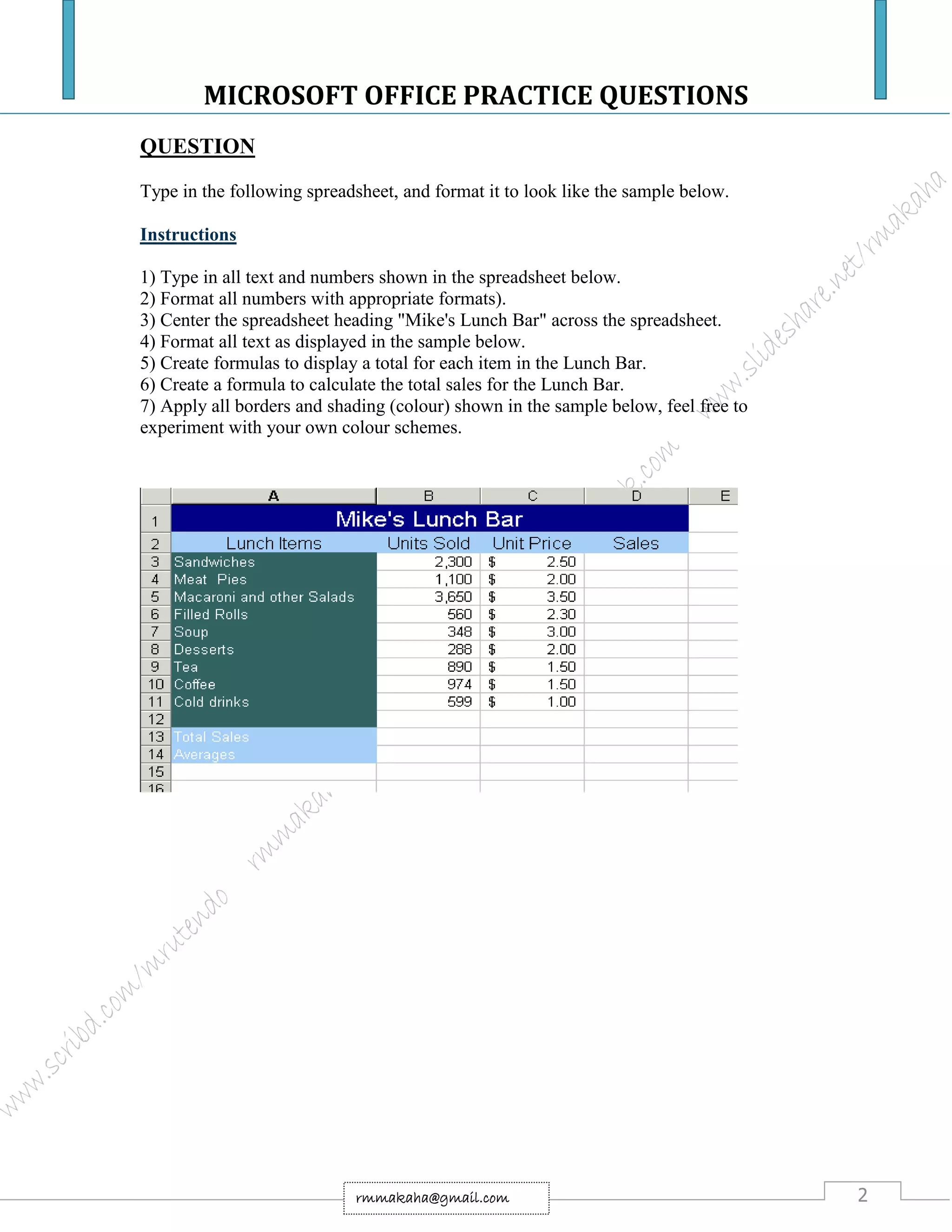
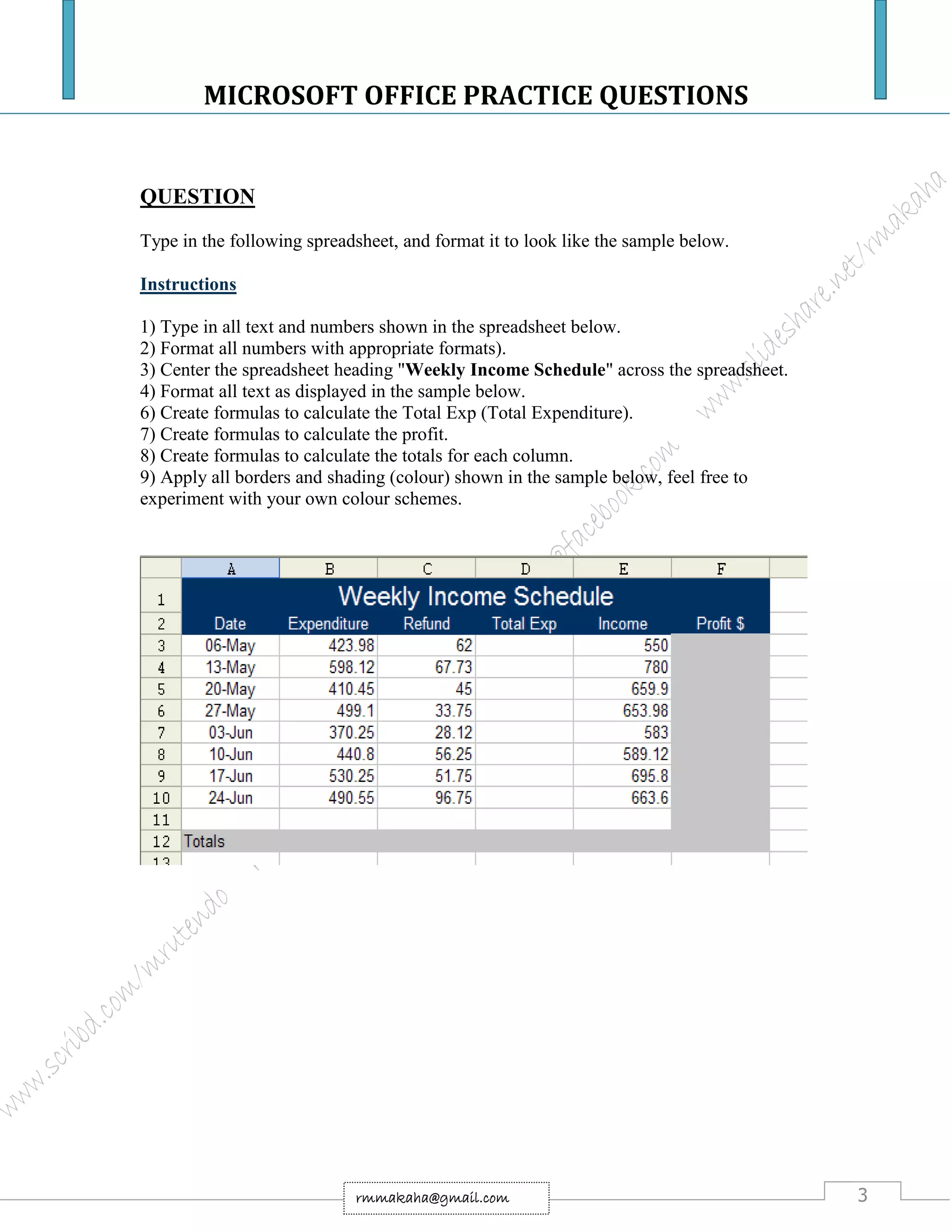
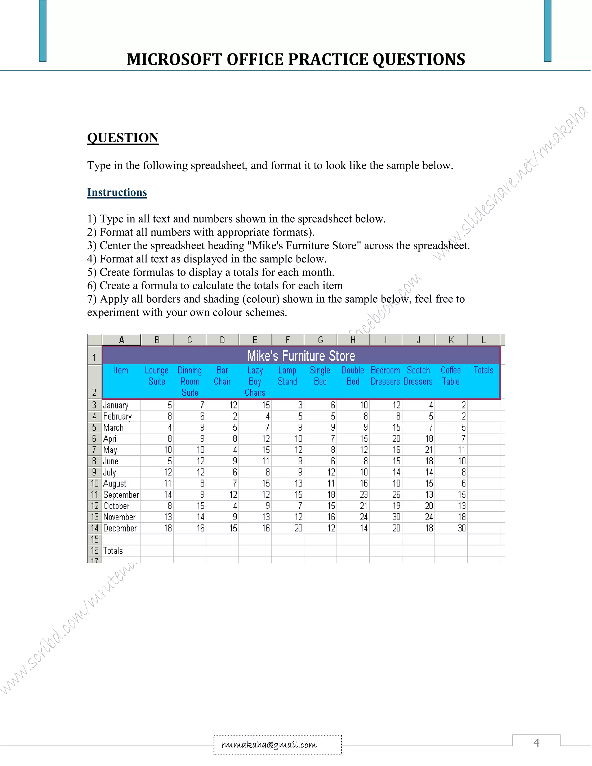
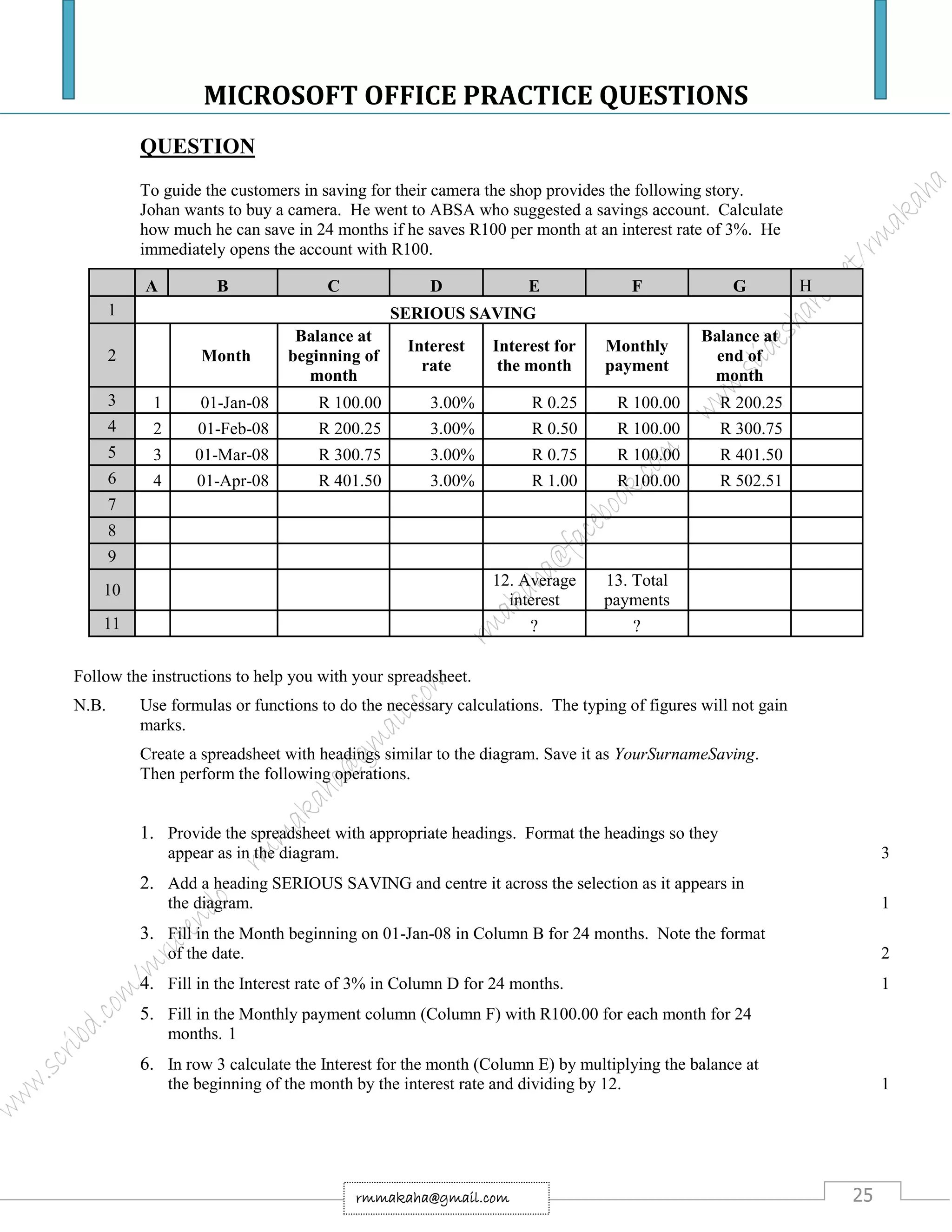
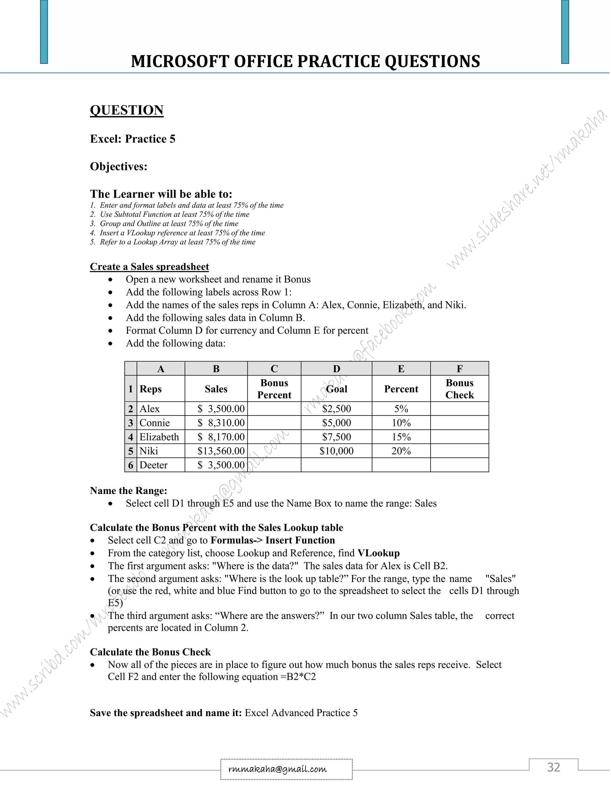
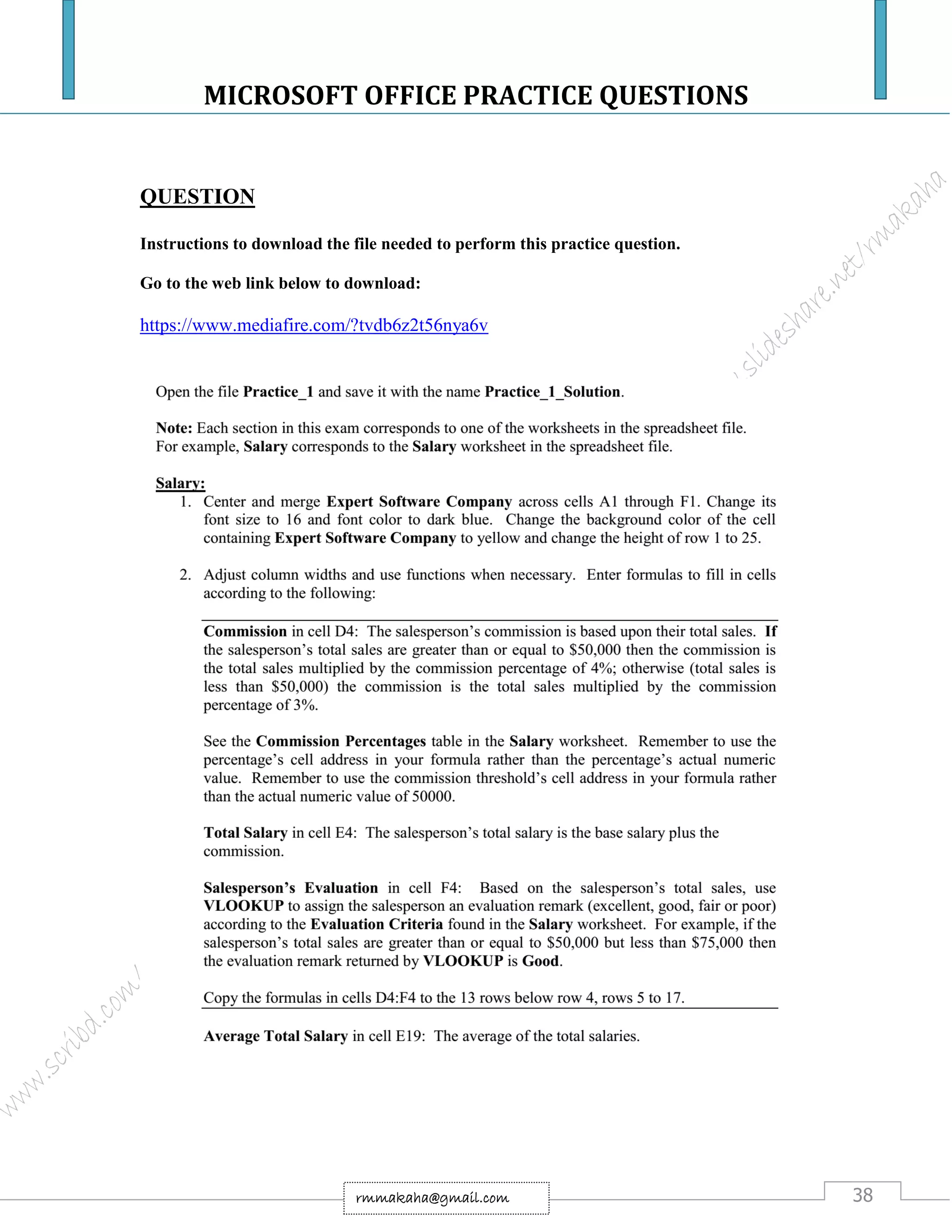
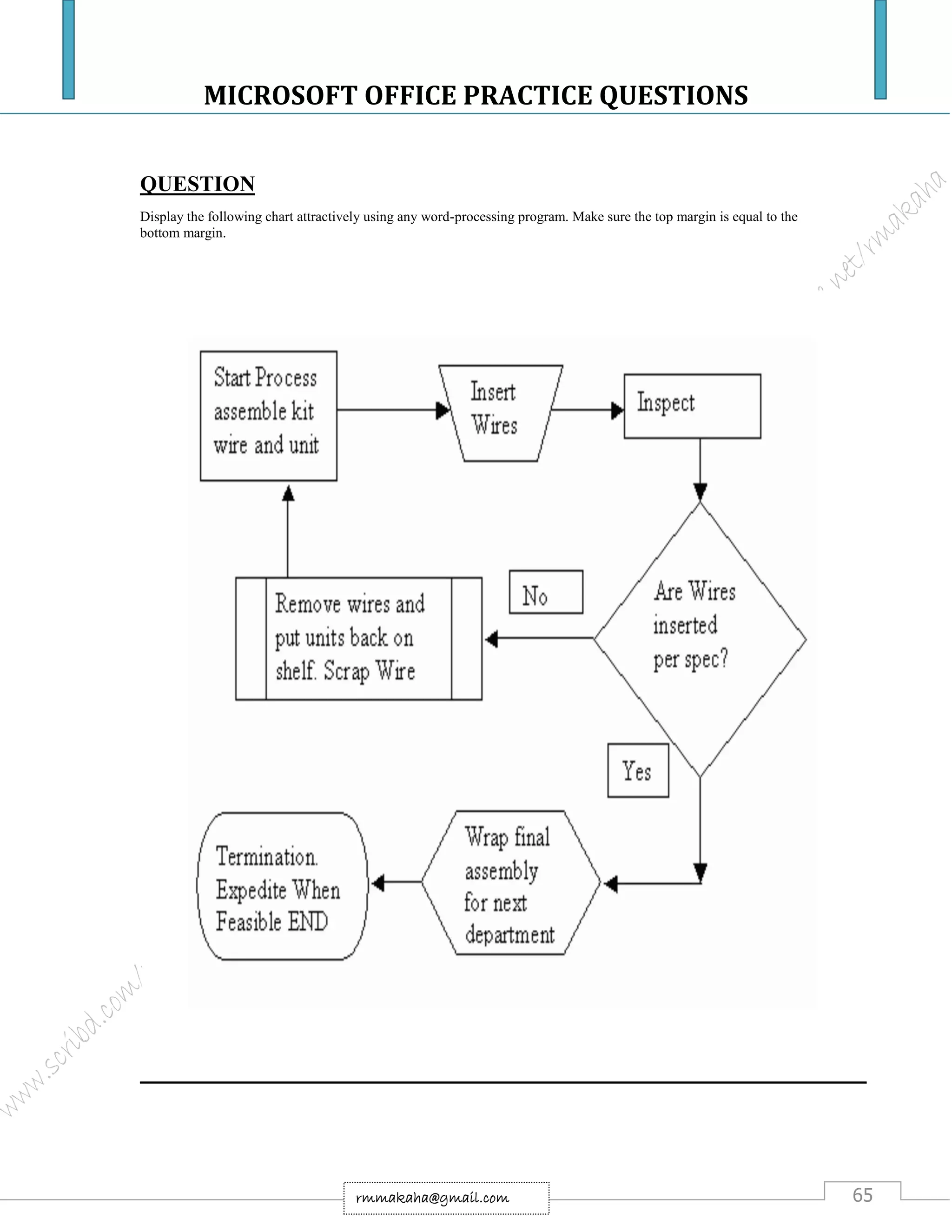
QUESTION
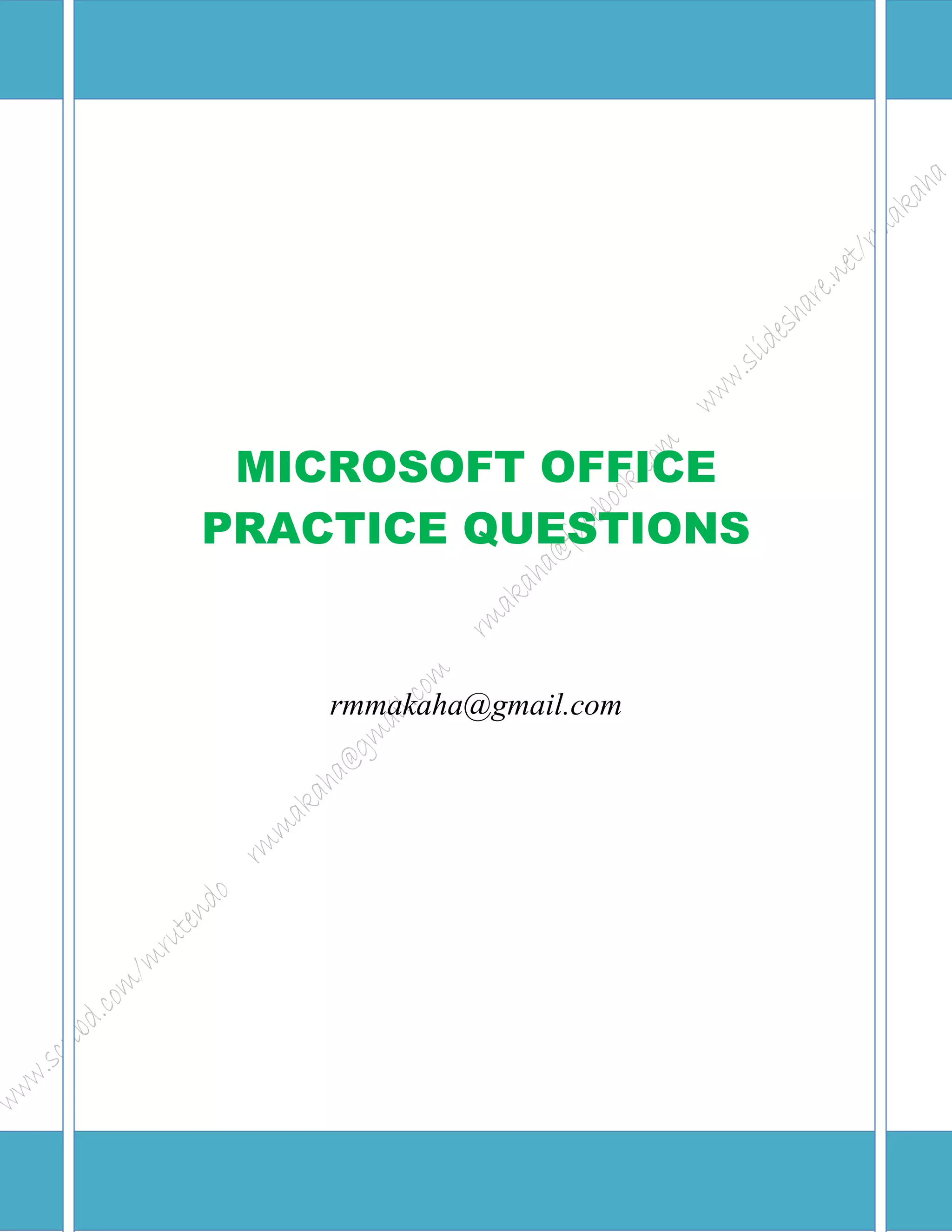
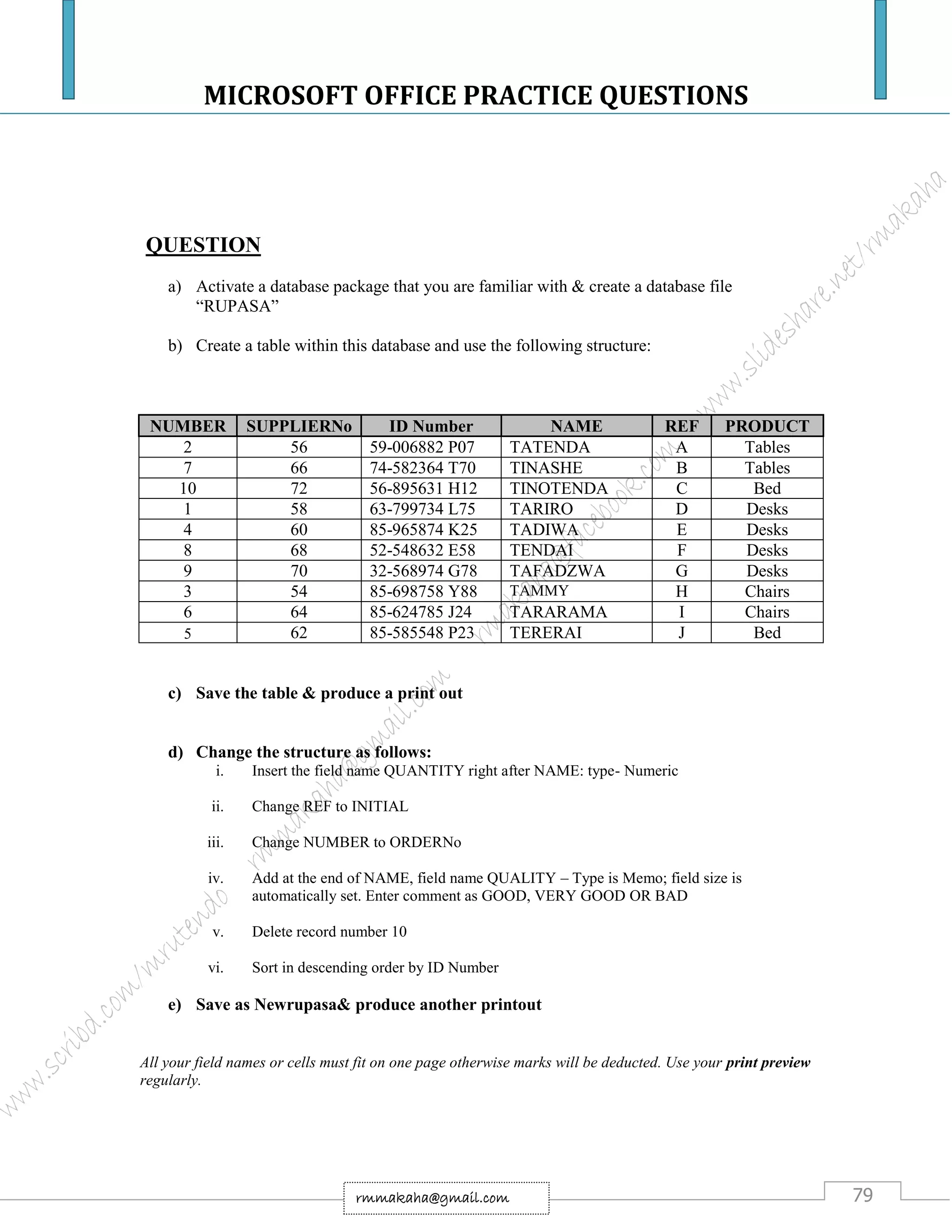
Using a spreadsheet package you have studied, construct T Morongo’s pay slip for December 2008
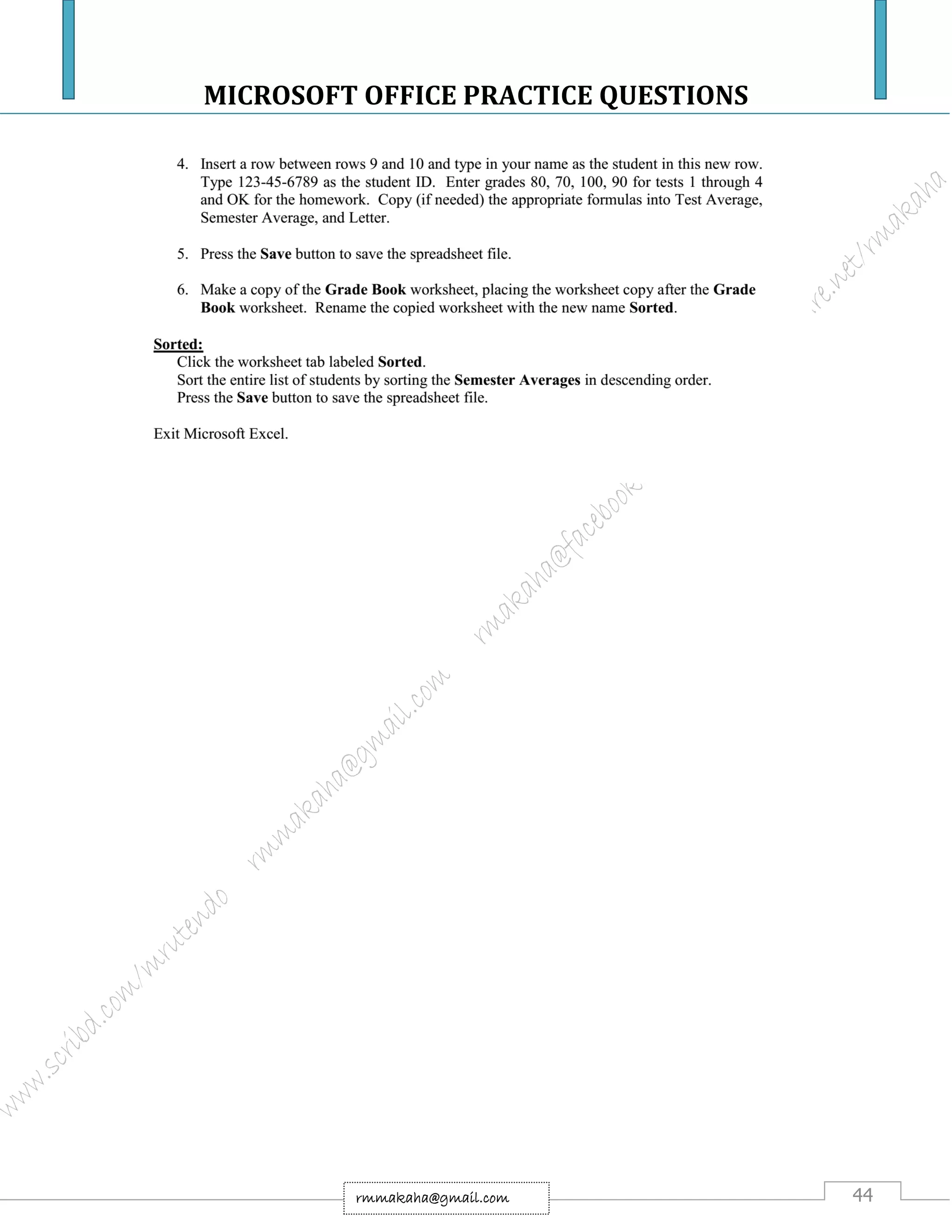
following the instructions below. Insert a custom footer with your name, subject, course, exam/Test &
question number. Save it as Salary advice. (5 marks)
SALARY ADVICE FOR DECEMBER 2010
EMPLOYEE : T MARONGO
STAFF NO. : 004
DATE : 31 DECEMBER 2010
NEXT PAY DATE : 31 JANUARY 2011
BASIC SALARY p.a.: $ 31200.00
INCOME AMOUNT DEDUCTIONS AMOUNT
Basic Salary Pension @ 8%
Housing Subsidy P.A.Y.E.
Vehicle Allowance U.I.F.
Medical Aid
Bond Repayment
Gross Income Total Deductions
Net Salary
INSTRUCTIONS
i. Housing Subsidy $6000 per year. [2]
ii. Car Allowance $100 per month.[2]
iii. Pension 8% on Basic Salary.[2]
iv. P.A.Y.E. $636.83 [2]
v. Medical Aid $70.[2]
vi. U.I.F 1% on Basic Salary + Housing Subsidy. [2]
vii. Bond Repayment $630.[2]
viii. Calculate Net Salary. [4]
ix. Format all figures to 2d.p. and insert a z$ currency symbol. [5]
x. Insert a custom footer with your name, subject, course, exam/Test & question number.
Save it as Salary advice2. [2]
All your field names or cells must fit on one page otherwise marks will be deducted. Use your print preview
regularly.

6rmmakaha@gmail.com
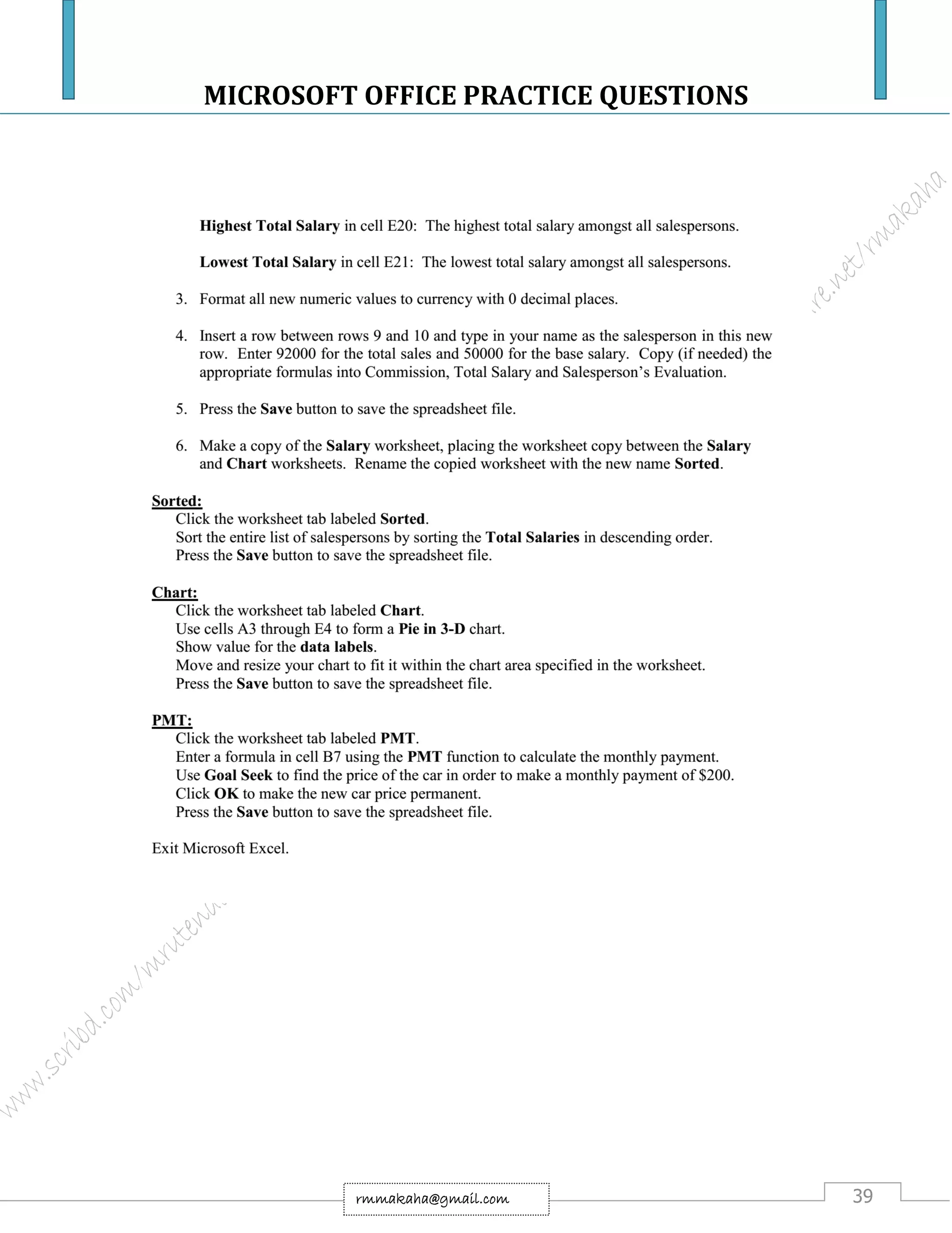
QUESTION
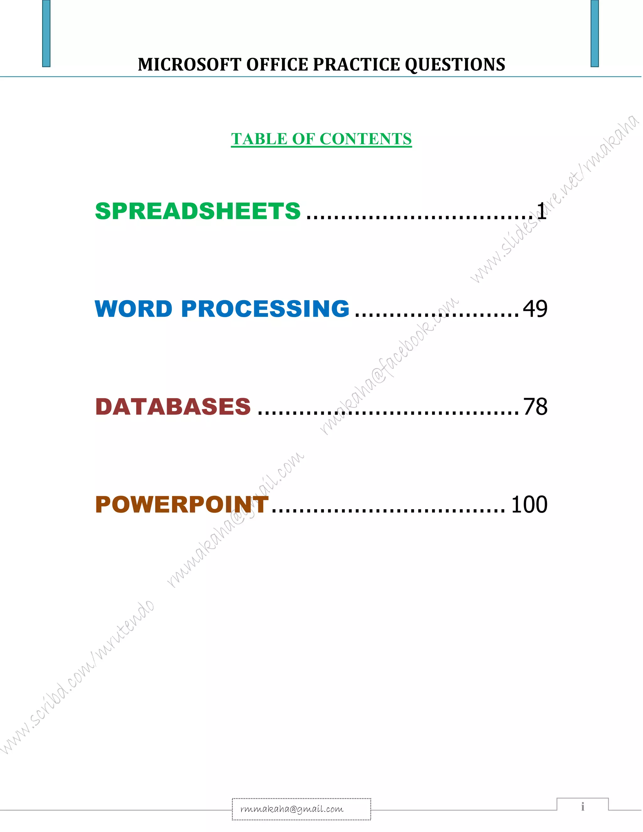
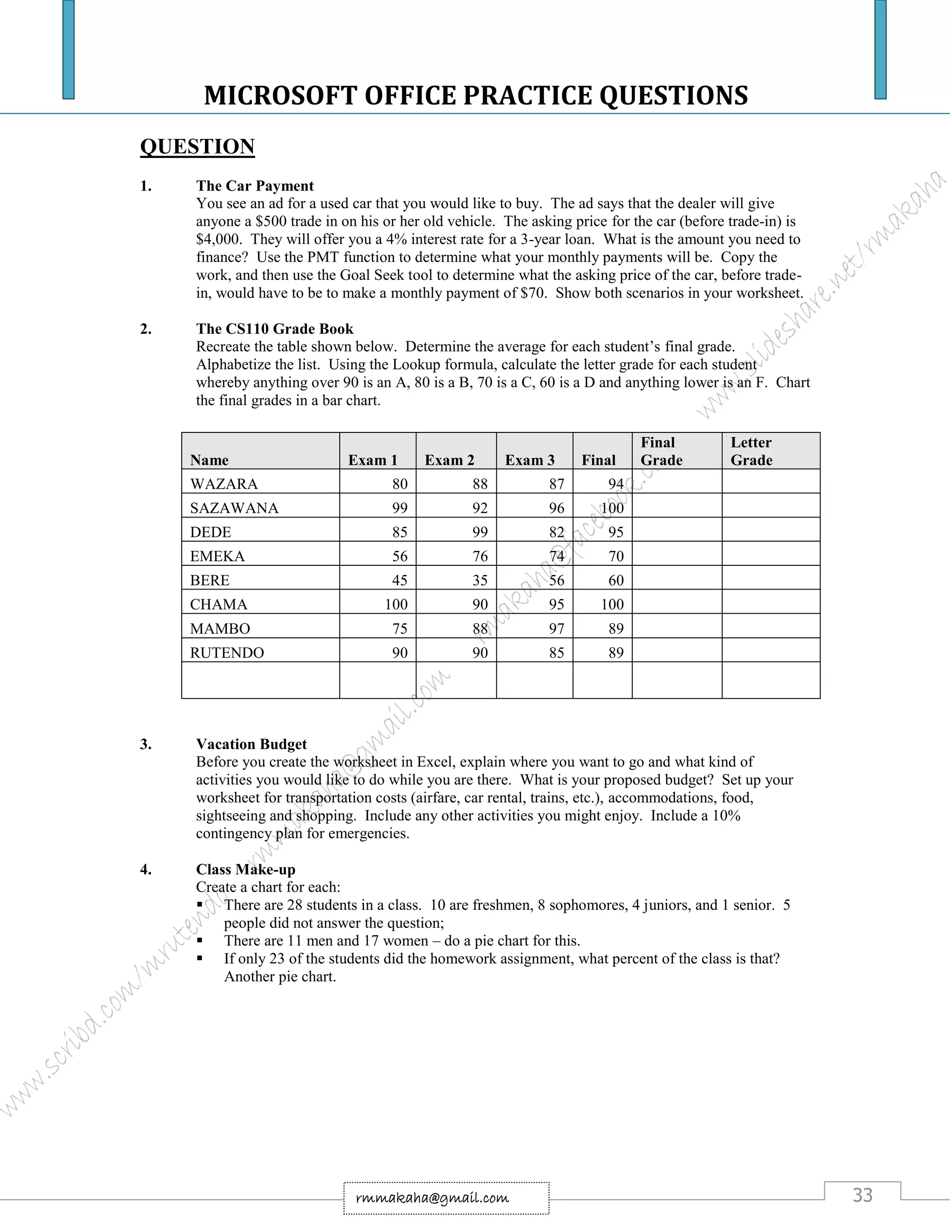
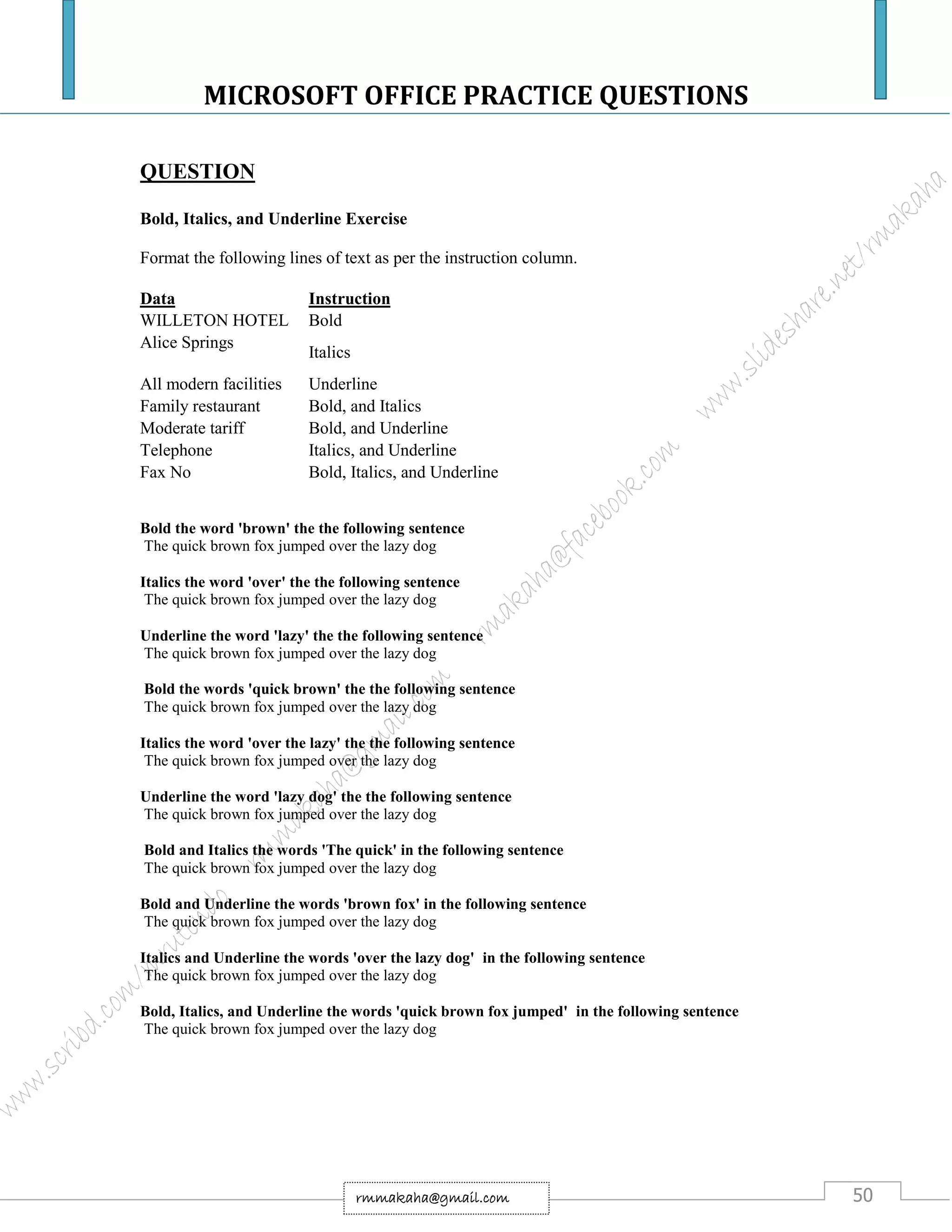
a) Create the following worksheet, in landscape format, produce a copy& save it as hotel. (5
marks)
Chibhanguza Hotel
EMPLOYEE NAME WORKED HOURS RATE PER HOUR
CHIHURI
CHINYERERE
MAKINA
MANYERE
MBASERA
CHIGIJI
ZUVA
KONDO
ANDERSON
59
66
95
78
55
98
123
100
88
220000
110000
330000
450000
250000
329000
222000
161000
176000
TOTAL
REQUIRED
b) Insert columns for Gross Salary, PAYE, Aids Levy, Housing allowance, Transport
allowance and Net Salary (2 marks)
c) Given that
o PAYE is 16%,
o Aids levy is 3%,
o Housing allowance is 15%,
o Transport allowance is 10% of Gross Salary.
i. Calculate the Gross salary,
ii. PAYE,
iii. Aids Levy,
iv. Housing allowance,
v. Transport allowance and
vi. Net Salary.(8 marks)
d) Calculate the totals and save the worksheet as Hotel 2. (2 marks)
e) Produce a column graph that shows Employee name and Net salary, save the worksheet
as colgraph. (5marks)
f) Show all formulas you have used in a new sheet. Adjust the column width so that the
formulae are displayed in full and the sheets fits into one side of A4 landscape format and
save it as formulas. [3 marks]
regularly.

7rmmakaha@gmail.com
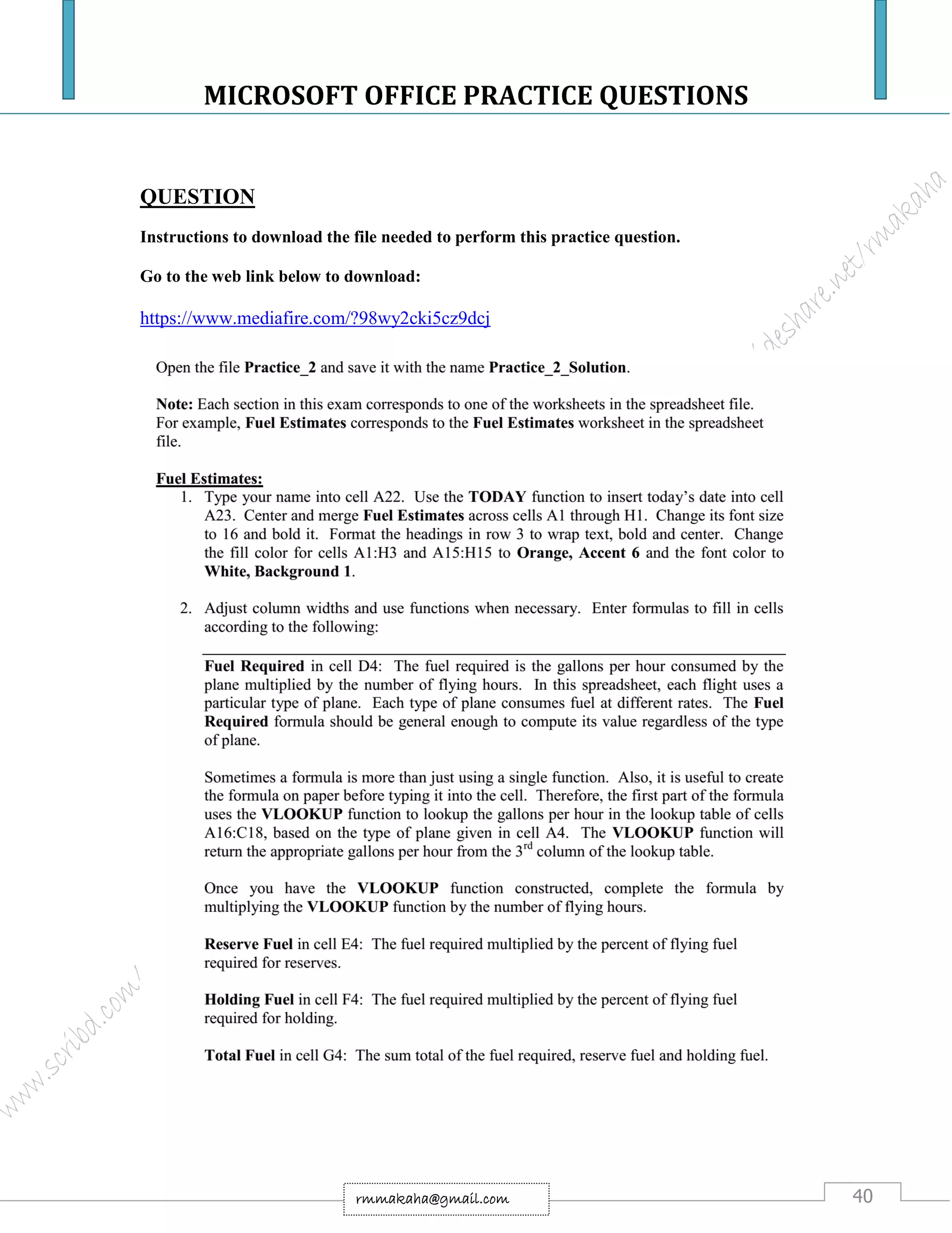
QUESTION
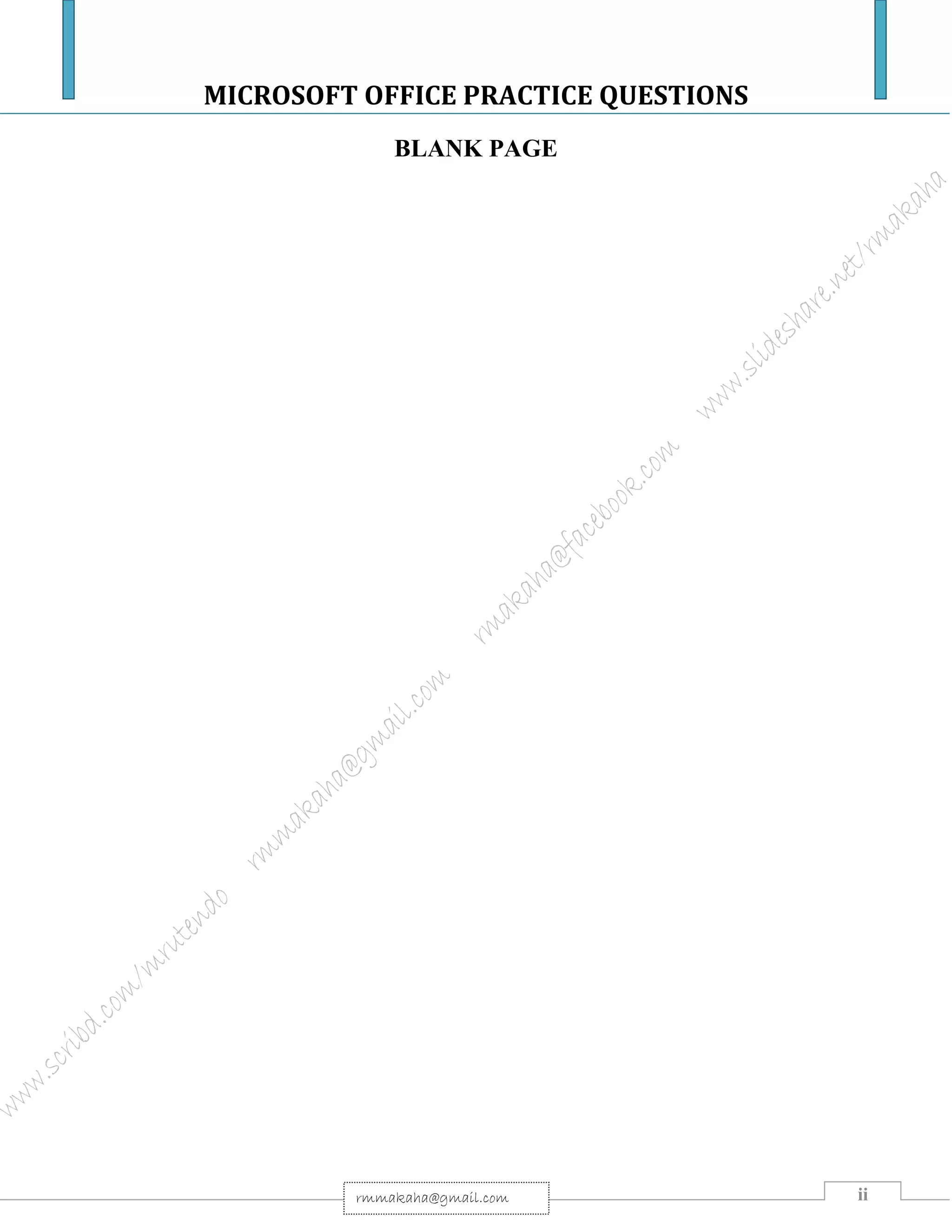
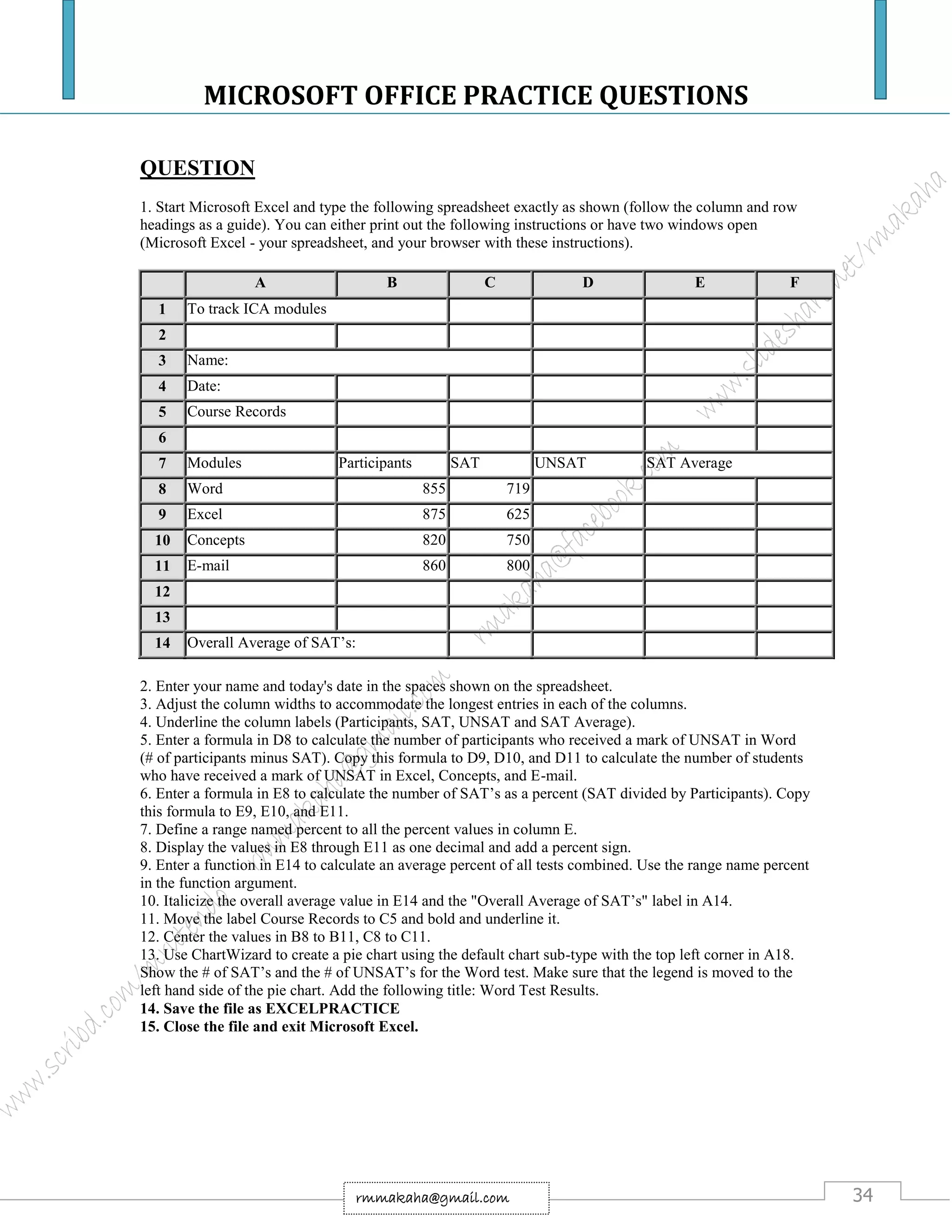
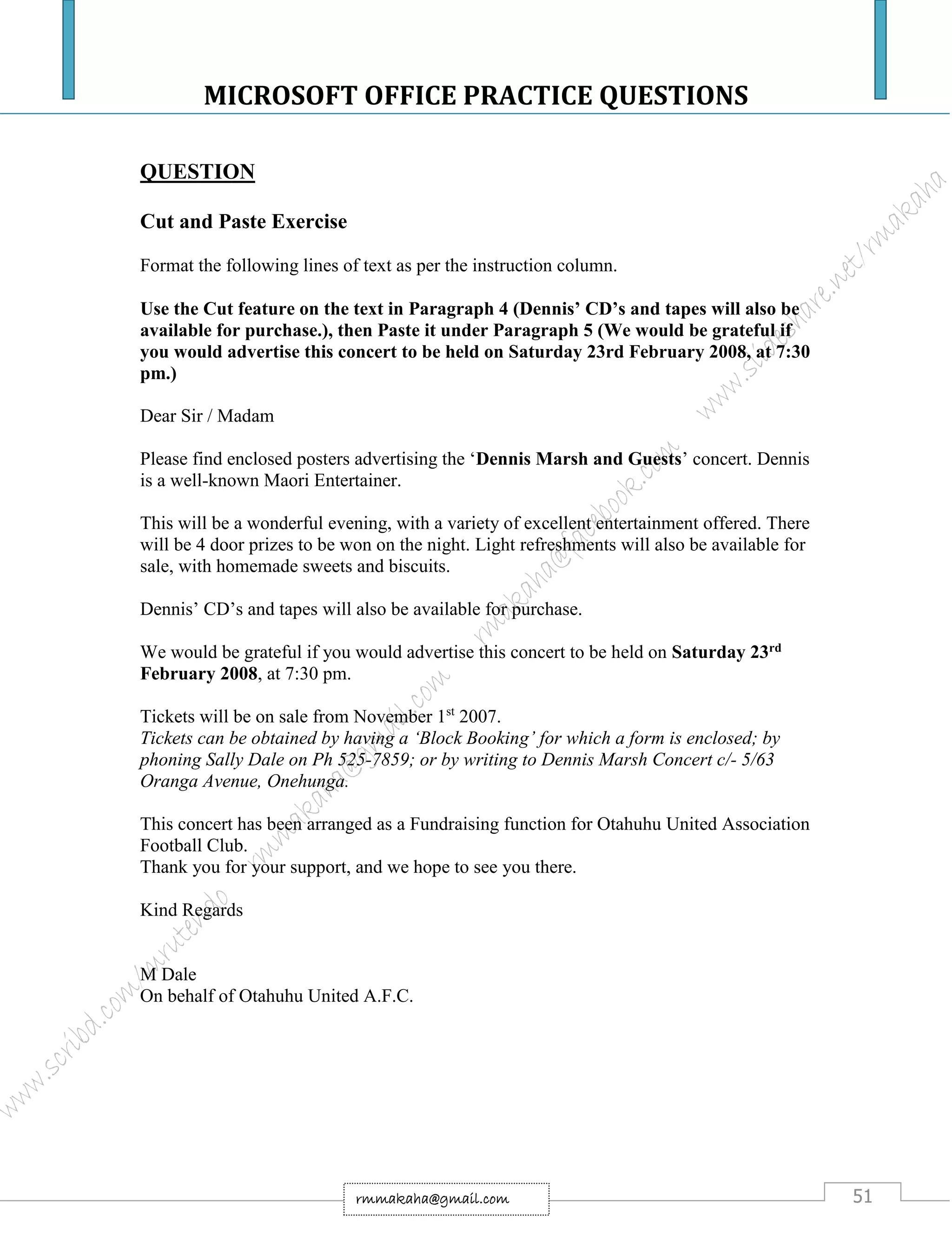
A furniture shop sells furniture to customers on credit. The credit terms request the
customer to make a deposit of 25%. The balance after the total deposit is paid in monthly
installments over 24 months without interest.
The shop customers & furniture credit values are:
Name Furniture value Deposit Balance Monthly installment
Farai
Itai
Sibongile
Isaac
Fundai
Shingai
Mary
$85 000.00
$55 000.00
$90 000.00
$63 700.00
$95 700.00
$65 800.00
$95 900.00
a) Design a spreadsheet of the data above& save it as Furniture. [3 marks]
b) Make all titles bold and shade the cell background for titles in light grey color. [3 marks]
c) Format the furniture value to zero decimal point. [2 marks]
d) Use formulae to calculate values for deposit, balance & monthly installments. [12 marks]
e) Sort the sheet in alphabetical order of names. [3 marks]
f) Insert borders on all entries & save the sheet as Furniture2 [2 marks]
g) ON A NEW SHEET, Create a fully labeled,
i. Column graph [5 marks]
ii. Bar Chart [5 marks]
iii. Pie Chart [5 marks]
Using the name and value of furniture columns & SAVE IT AS GRAPHS.
h) Show formulas you have used for deposit, balance & monthly installment in a new sheet
and save it as formulas. [10 marks]
regularly.

8rmmakaha@gmail.com
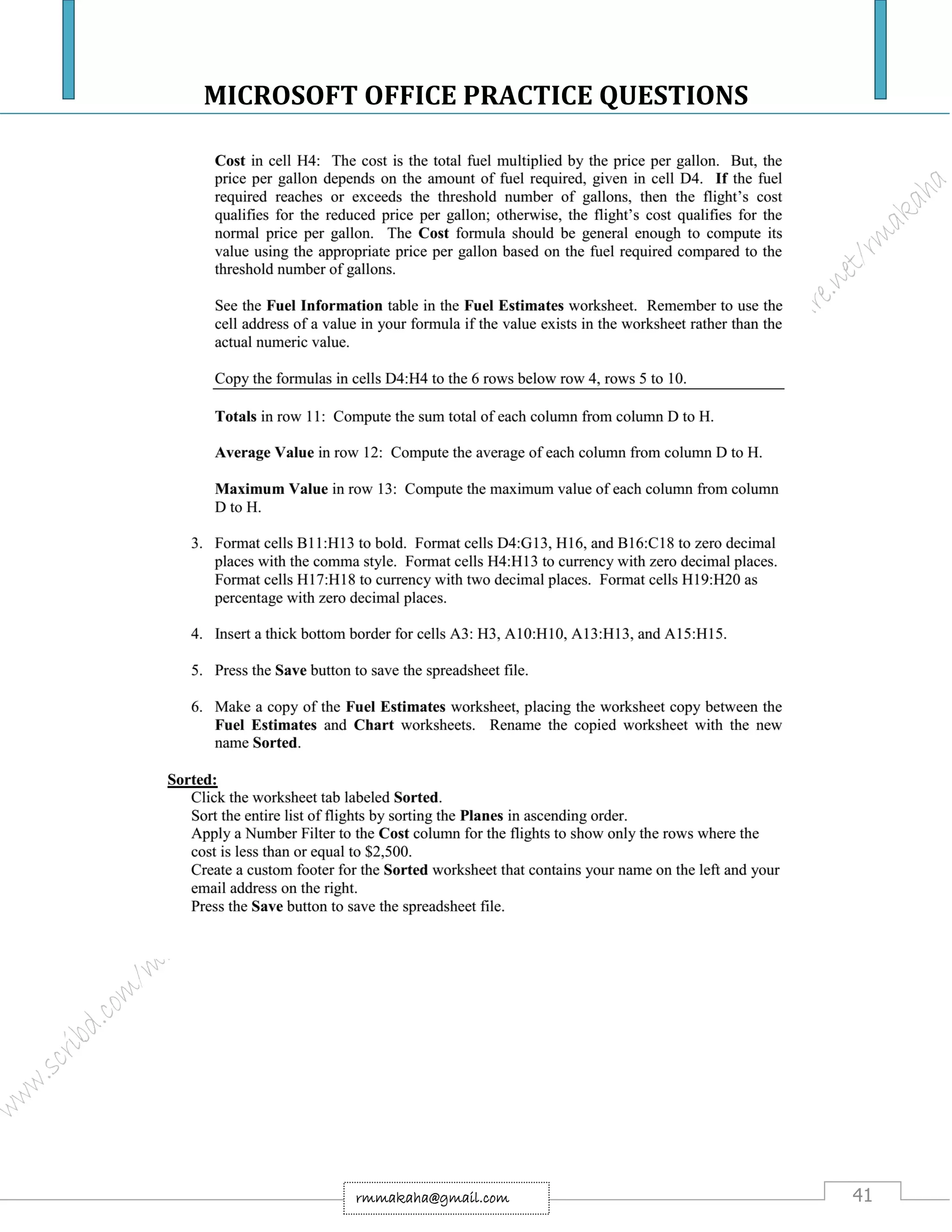
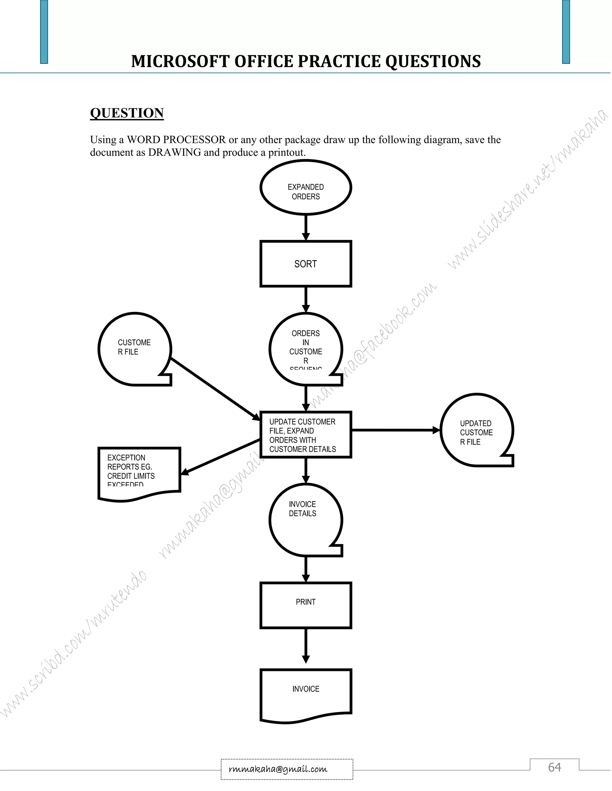
QUESTION
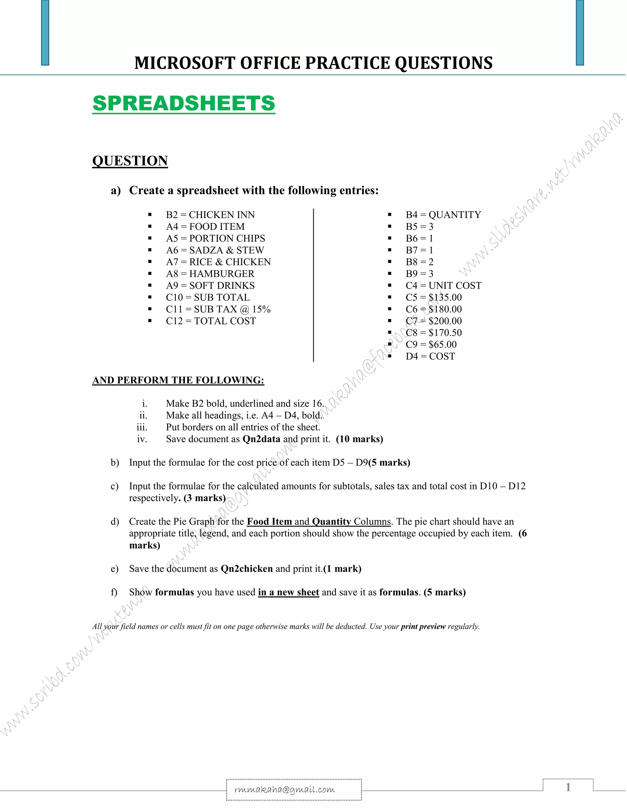
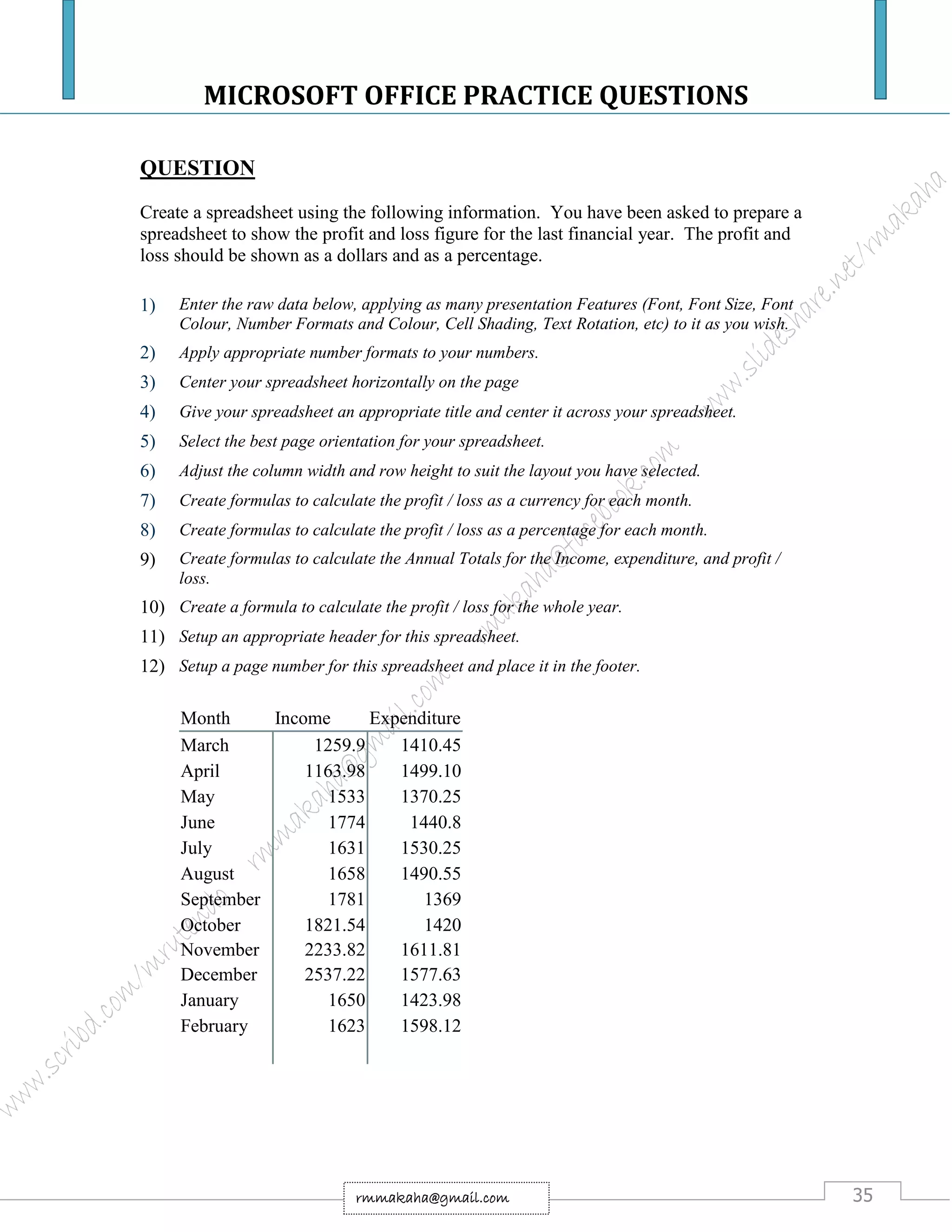
a) Create a spreadsheet with the following entries & save it as ENG1 [5 marks]:
ENGINEERS’ SALARIES
Engineer’s Name Hours worked Rate per hour Salary
Eng. Mudehwe
Eng. Bejera
Eng. Mudzuri
Eng. Muzawazi
Eng. Zhawari
Eng. Mutekede
180
300
500
200
300
120
$1000
$2000
$2500
$1500
$2500
$2000
Perform the following:
a. bold & underline the title [2 marks]
b. make all heading bold [2 marks]
c. put borders on all entries of the sheet [ 2 marks]
d. Save the worksheet & print it. [ 1 mark]
b) Given that salary = hours worked multiplied by rate per hour, calculate the salary. [6
marks]
c) Add the following Engineers to the worksheet: [2 marks]
Eng. Mavhunga
Eng. Bepete
500 hours
600 hours
$3000 per hour
$3500 per hour
d) i) Calculate the total number of hours worked & the total amount paid to all the
Engineers. [ 4 marks]
ii) Format rate per hour & salary to zero decimal point. [1 mark]
e) Create a pie chart for the Engineers’ names & the hours worked columns. The pie
chart should have an appropriate title legend and each portion should show the
percentage of hours accumulated by each Engineer. [5 marks]
Save the worksheet & print it.
f) Show all formulas you have used in a new sheet, and save it as formulas. [10 marks]
regularly.

9rmmakaha@gmail.com
QUESTION
COURSEWORK MARKSHEET
a) Using a spreadsheet package you have learnt, type the above mark sheet. Save as
marks and print a copy. (10 Marks)
b) Calculate the missing figures (1 decimal point) using formulae. Save as marks2
and print a copy. (15 marks)
THEORY PRACTICAL
TESTS ASSIGNMENTS ASSIGNMENTS
NAMES 1 2 20% 1 2 15% 1 2 25%
MAKWIRO 73 55 - 89 50 - 90 60 -
GORONGA 74 55 - 75 54 - 85 65 -
BANGO 77 55 - 70 63 - 80 70 -
MAKAHA 55 73 - 66 65 - 75 75 -
MEKI 60 58 - 70 70 - 60 92 -
MAPHOSA 85 51 - 40 63 - 75 80 -
MADI 63 - 53 83 - 75 85 -
LIMA 50 53 - 29 39 - 50 63 -
DAUDI 75 41 - 70 61 - 59 49 -
AVERAGE
HIGHEST
LOWEST

10rmmakaha@gmail.com
QUESTION
Please set up a spreadsheet using the following information. Do not put any lines or
borders on it yet.
Names Weight
peaches
Weight plums Weight
oranges
Total weight
80Linda
73Joseph
01Rufaro
78Simbai
85Langton
100
34
25
164
290
50
212
25
167
0
0
21
33
74
3
i. Save it as Qn-fruits1. [5 marks]
ii. Use the Sum formula to calculate the Total weight (kg) of fruit packed by each worker. [5 marks]
iii. Format all the numbers as integer (2 decimal places). [1 mark]
iv. Separate employee names & their payroll numbers, by inserting 2 columns after the Names column & insert
the headings Employees & Payroll Number. Enter the information into the 2 columns. (See example
below).
Employees Payroll Number
Linda
Joseph
Etc
80
34
Etc
v. Center align the Payroll Number heading & the numbers in the column. (1 mark)
vi. Delete the Names column (1 mark)
vii. Add a title WEEKLY PRODUCTION FIGURES in bold, font size 16 above the spreadsheet. [2 marks]
viii. Add rows at the bottom of the worksheet and label them AVERAGE, MAXIMUM & MINIMUM. [3 marks]
ix. Calculate the average, maximum & minimum values for the columns containing weights only. [6 marks].
x. Add shading to the column headings and borderlines to the full table. (Include the column headings but not
the title in the border). [2 marks]
xi. Set up the spreadsheet ready for printing in landscape format [1 mark].
xii. Save the worksheet as Qn-fruit2. [1 mark]
xiii. Create a pie chart titled (EMPLOYEE PAYROLL NUMBERS) for the Employees & Payroll Number
columns only. Do not show a legend on your chart. Data labels indicating percentages should be displayed.
Display the chart as a new sheet & print it. [5 marks]
xiv. Change the spreadsheet to display formulae you have used. Adjust the column width so that the formulae are
displayed in full and the sheets fit into one side of A4 landscape format. Save the worksheet as formulas in
landscape format. [5 marks]
regularly.

QUESTION
Use a new workbook & construct a worksheet with the data given & save it as LYONS.
[5 marks]
LYONS INC.
Orange JUICE sales
PRODUCT COST
PRICE
PER
LITRE
MARK UP
PER ITEM
35%
SELLING
PRICE
LITRES
SOLD
TOTAL
INCOME
PROFIT
Cascade
Quench
Xtra
Sun Splash
House brand
3.75
3.65
4.25
1.50
1.50
234
345
456
123
245
TOTAL
AVERAGE
HIGHEST
LOWEST
INSTRUCTIONS
 Markup= Cost price/Litrex 35%
 Selling price= Cost price/Litre + Mark up
 Total income= Litres sold x Selling Price
 Profit = Total income – (Cost price/LitrexLitres sold)
a) The MARKUP % (35%) must be inserted in a separate cell under the heading. USE IT as an
absolute cell reference in the formula to calculate the markup per item. [6 marks]
b) Calculate the mark up for each item. [5 marks]
c) Calculate the selling price for each item. [5 marks]
d) Calculate the Total Income for each item. [5 marks]
e) Calculate the profit for each item. [5 marks]
f) Format the column LITRES SOLD to display the number of litres as integers. The rest of the
worksheet must be formatted to display two decimals. [4 marks]
g) Use statistical functions to calculate the:
o AVERAGE
o HIGHEST (MAX)
o LOWEST (MIN) for Selling Price column up to Profit Column. [6 marks]
h) Show all formulas you have used in a new sheet. Adjust the column width so that the
formulae are displayed in full and the sheets fits into one side of A4 landscape format and
save it as formulas. [10 marks]
i) Under the worksheet Create a pie chart titled PRODUCT COST PER UNIT for Product &
Cost price per Litre columns. Data labels indicating percentages should be displayed. [5
marks]
j) Put borders neatly on the on the work sheet & save it as LYONS2. [4 marks]
regularly.

QUESTION
a) Reproduce the following worksheet & save it as monthly sales, insert a title Half
Yearly Sales & produce a print out (5 marks)
Names January February March April May June
Mr. Dube 20000 10000 1000 100000 60000 150000
Mr. Moyo 25000 12000 8000 200000 50000 250000
Mr. Sibanda 30000 18000 16000 300000 40000 350000
Ms Ncube 35000 22000 32000 400000 30000 450000
Ms Sibanda 20000 20000 23000 22000 23000 240000
Mr. Zuze 40000 24000 64000 500000 20000 650000
Mr. Jazi 45000 28000 128000 600000 10000 750000
Mr. Mugara 50000 32000 4000 700000 70000 850000
Mrs.Madyira 55000 34000 12000 800000 80000 950000
Mr. Kotso 60000 40000 74000 900000 90000 200000
TOTAL - - - - - -
AVERAGE - - - - - -
HIGHEST - - - - - -
LOWEST - - - - - -
b) Calculate the missing figures using formulae & embolden them. (12 marks)
c) Produce a column graph on a new sheet showing the heading Monthly sales for 6
months. [4 marks]
d) Print the worksheet with formulae & save it as formulae. It should fit on one sheet. [4
marks]
regularly.

QUESTION
a) Reproduce the following worksheet & save it as IT-Costing, insert a title Computer
Consumables Costing & produce a printout (5 marks)
Product
Description
Cost price Mark
up
Selling
price
Gross
profit
Storage
Expenses
Net
Profit/loss
40 GB disk
Drive
CD Writer
TV Tuner Card
Sound Card
Video Card
Multimedia
Speakers
Keyboard
Mouse
Mouse pad
800000
1300000
1500000
300000
800000
400000
100000
250000
80000
10000
12000
10%
20%
15%
20%
15%
30%
20%
20%
25%
20%
10%
5000
120000
110000
40000
30000
25000
12000
15000
18000
9000
10000
Total
b) Insert the currency symbol on cost price, selling price, gross profit, totals & net profit/
loss and format to 2 decimal places. (5 marks)
c) Use given mark up percentages & calculate the selling price, gross profit, net profit &
totals. Save the worksheet as IT-costing2 & produce a print out.
(15 marks)
d) Change the spreadsheet to display formulae you have used. Adjust the column width so
that the formulae are displayed in full and the sheet fits into one side of A4 landscape
format. Save the worksheet as formulas in landscape format. [5 marks]
regularly.

QUESTION
a) Create a worksheet using data below & save it as Sales& produce a print out.
[3 marks]
Product Percentage Sales
Mouse
Keyboards
Hard disks
CD-ROMs
Floppy disks
Sound Cards
CD-R
Monitors
10
12
8
10
20
8
12
20
b) Create a pie chart using the data above. On the chart put/ Display Data labels indicating label &
percent. [3 marks]
c) The chart title should be: COMPUTER CONSUMABLES PERCENTAGE SALES. It should be
inside the chart (font type: Agency FB & font size 14, underline the title). [3 marks]
d) Format the legend font type to Agency FB & font size to 8. Reduce the size of your legend if it is
coming to contact with the Chart title. [3 marks]
e) Format data labels font size to 10 & font type to Agency FB or Arial narrow. [3 marks]
f) Using your print preview make your pie chart large & fitting. Save your pie chart as Piesales [5
marks]
g) Create a worksheet from the following data & save it as cellphones print copy
[3 marks]
h) Create a Column chart from the data above. Use the first chart sub-type.
[3 marks]
i) Insert a chart title: CELLPHONES PRICE GRAPH. It should be inside the chart (font type: Algerian
& font size 14, underline the title). [3 marks]
j) Format the legend font type to Agency FB & font size to 8 & bold it. [3 marks]
k) Label the X-axis (Mobile Type) & Y-axis (Amount (Z$)), & the font type of the X & Y-axis to
Agency FB, size 10. [8 marks]
l) Using your print preview make your column graph large & fitting. Make sure every cell phone or
mobile name is appearing on your graph. Save your column graph as Cellbar& print a copy. [5
marks]
m) Print a directory listing. [5 marks]
regularly.
Cell phone Price ($)
Nokia 5510
Sagem 300
Nokia 3330
Philips C50
Nokia 3410
Nokia 2110
Motorola C300
Siemens A50
Samsung 200
500
2500
3000
4500
5000
4000
3500
2000
1000

QUESTION
a) The following data shows gasoline consumption rates for different cars traveling at different
speeds. Create a worksheet using the data, save it as cars & produce a print out. (5 marks)
60km/h 120km/h 160km/h
Benz
Mazda
VW
Toyota
BMW
Lexus
Mitsubishi
Honda
80
70
60
50
40
30
20
15
90
80
70
60
50
40
30
25
100
90
80
70
60
50
40
35
b) Insert a title GASOLINE CONSUMPTION FOR DIFFERENT MAKES OF CARS at the
top of the worksheet. [2 marks]
c) Produce a gasoline consumption column graph, with a relevant Chart title, X & Y –axis & a
proper legend for the data. The candidate is reminded to use print pre-view to make sure his/
her graph fits on the page. [8 marks]
d) Insert between Toyota & BMW details of the following car: [5 marks]
Nissan 45 55 65
e) Save as cars2 &produce a print out.
f) Create a worksheet using the data below & save it as Employees. [5 marks]
Name Surname Employee # Gross Wage Deductions Net
wage
Aim
Zexel
John
Mark
Terry
Xavier
TOTAL
Green
Blue
Gray
Purple
Metros
Jones
Aa500
Bb510
Cc520
Dd530
Ee540
Ff560
100000
250000
600000
300000
200000
650000
25000
45000
95000
35000
30000
10000
g) Underline & embolden the heading. [1 mark]
h) Format the wage columns to currency for the dollar sign to appear. [4 marks]
i) Use appropriate formulae to calculate the Net Wage, Total Deductions, Total Net Wage &
Total Gross Wage. [10 marks]
j) Save as Employee2
regularly.

QUESTION
COURSEWORK MARKSHEET
a) Using spreadsheet package you have learnt, design the above mark sheet & save it as
MARKSHEET. [6 marks]
b) Calculate the missing figures using formulas [embolden the missing figures] & save the sheet as
NEWMARKSHEET. [14 marks]
c) Insert a chart as new sheet showing: NAMES, TEST MARKS, THEORY ASSIGNMENT, &
PRACTICAL ASSIGNMENTS & save it as MARKCHART. [5 marks]
d) Change the spreadsheet to display formulae you have used. Adjust the column width so that the
formulae are displayed in full and the sheet fits into one side of A4 landscape format. Save the
worksheet as formulas in landscape format. [5 marks]
regularly.
THEORY PRACTICAL
TESTS ASSIGNMENTS ASSIGNMENTS 60% INT.60%
NAMES 1 2 20% 1 2 15% 1 2 25%
NYONI A. 73 55 - 89 50 - 90 60 - - -
GUNYEKU M. 74 55 - 75 54 - 85 65 - - -
BIKWA K. 77 55 - 70 63 - 80 70 - - -
MAKEDENGE
C. 55 73 - 66 65 - 75 75 - - -
DHANERA M. 60 58 - 70 70 - 75 80 - - -
GARA X. 85 51 - 40 73 - 75 85 - - -
Average - - - - - - - - - - -
Highest - - - - - - - - - - -
Lowest - - - - - - - - - - -

QUESTION
Create the following worksheet.
MEAT
TYPE
NO. OF
KGS
PRICE/KG TOTAL
COST
VAT COST +
VAT
DICOUNT
ALLOWED
NET COST
BLADE 21.20 28400
FILLET 112.39 21200
BRISKET 89.70 36400
LIVER 150 8500
REQUIRED
a) Below the worksheet enter the following headings & calculate:
i. Average number of kg’s. [1 mark]
ii. Highest discount allowed. [1 mark]
iii. Lowest value added tax. [1 mark]
b) i. Value Added Tax 15% of total cost. Calculate the VAT. [2 marks]
ii. Discount Allowed is 3.5% of cost plus tax. Calculate. Discount Allowed. [2 marks]
iii. Calculate the Net Cost. [2 marks]
iv. Calculate the total cost. [2 marks]
c) Round off the entries for total cost to 2 decimal places. [1 mark]
d) Include the currency symbol in the Net Cost Column (use the ‘$’ sign). [1 mark]
e) Column headers to be Arial font type, size 11, bold & italics. [2 marks]
f) Insert the title “Premier Meat Sales” at the top of the worksheet. [ 2 marks]
g) For the title to be Arial font type, size 14, color white, with a black background. [2 marks]
h) Set the worksheet to landscape format & save the worksheet as “CONFIDENTIAL”.
[3 marks]
i) Save the worksheet with formula as “CONFIDENTIAL1”. Print it in landscape orientation. [3 marks]

QUESTION
a) Reproduce the following worksheets as they are, & save them separately as
TPL-acc & Bsheet. [15 marks]
T Bejera
Trading & Profit & Loss Account for the year ended 31 December 2025
Sales
Return inwards
Less cost of goods sold
Opening stock
Purchases
Return outwards
Closing stock
GROSS PROFIT
Discount received
Less: Expenses
Wages & salaries (8940+210)
Rent & insurance (1740-180)
Carriage Inwards
General expenses (450+20)
Discount allowed
Provision for bad debts
Depreciation: Fixtures
: Delivery Van
NET PROFIT
22860
570
120
300
41970
810
5160
Formulae
Formulae
4290
?
?
2160
?
1440
150
Formulae
Formulae
Formulae
Formulae
930
Formulae
Formulae
Formulae
All your field names or cells must fit on one page otherwise marks will
be deducted. Use your print preview regularly.

T Bejera
Balance sheet as at 31 December 2025
FIXED ASSETS
Fixtures & Fittings
Delivery Van
CURRENT ASSETS
Stock
Debtors
Prepaid expenses
Cash in hand
Less: CURRENT LIABILITIES
Creditors
Expenses owing
Bank overdraft
FINANCED BY:
Capital
NET PROFIT
Drawings
COST
Formulae
2100
Formulae
11910
Formulae
6060
230
4350
ACCUMULATED
DEPRECIATION
120
300
Formulae
4290
1100
180
90
Formulae
Formulae
NET BOOK
VALUE
108
Formulae
Formulae
Formulae
Formulae
7200
?
Formulae
2880
Formulae
b) Using your Basic Accounting knowledge, where you typed in formulae, put the
actual formulas & where you inserted a ? Put the required figure & save the
worksheets as TPL-acc2 & Bsheet2 respectively. [25 marks]
c) Show all formulas you have used in the TPL account & the balance sheet separately
in new sheets, named, TPL-formulas & BS-formulas respectively. The formulae
should fit on respective sheets. [10 marks]
regularly.

QUESTION
a) Reproduce the following worksheets as they are, & save them separately as
TPL-acc & Bsheet. [15 marks]
T MORGAN
Trading & Profit & Loss Account for the year ended 31 December 2025
Sales
Return inwards
Less cost of goods sold
Opening stock
Purchases
Return outwards
Carriage inwards
Closing stock
GROSS PROFIT
Discount received
Less: Expenses
Wages & salaries
Rent (25973-1120-5435)
Heating (11010+1360)
Carriage outwards
Advertising
Postage & Telephone
Bad Debts
Discount allowed
Depreciation
NET PROFIT
135680
13407
259870
Formulae
15654
Formulae
11830
Formulae
17750
38521
?
?
4562
5980
2410
223
2008
2306
12074
254246
Formulae
Formulae
1750
Formulae
Formulae
Formulae

T MORGAN
Balance sheet as at 31 December 2025
FIXED ASSETS
Fixtures & Fittings
CURRENT ASSETS
Stock
Debtors
Prepaid expenses
Bank
Cash in hand
Less: CURRENT LIABILITIES
Creditors
Expenses owing
FINANCED BY:
Capital
NET PROFIT
Drawings
COST
Formulae
24500
Formulae
19840
1360
ACCUMULATED
DEPRECIATION
63020
17750
23765
6555
4440
534
Formulae
Formulae
NET BOOK
VALUE
57720
Formulae
Formulae
83887
?
Formulae
18440
Formulae
b) Using your Basic Accounting knowledge, where you typed in formulae, put the actual
formulas & where you inserted a ? Put the required figure & save the worksheets as TPL-
acc2 & Bsheet2 respectively. [20 marks]
c) Show all formulas you have used in the TPL account & the balance sheet separately in new
sheets, named, TPL-formulas & BS-formulas respectively. The formulae should fit on
respective sheets. [10 marks]

QUESTION
a) Using MS Excel draw up a trading and profit and loss account for the
year ended 31 December 2006, & A BALANCE SHEET AS AT THAT
DATE in a new worksheet. 4 Columns should be used, 1 for details and
the other 3 for the figures. The columns for the figures should have 4
borders. Underline where necessary using a cell border. USE
FORMULAS FOR ALL CALCULATIONS. [20 marks]
Sales
Return inwards
Cost of goods sold
Opening stock
Purchases
Return outwards
Closing stock
Gross profit
Discount received
Wages & salaries
Rent & insurance
Carriage outwards
General expenses
Discounts allowed
Depreciation: fixtures & fittings
Delivery van
NET PROFIT
41970
810
?
5160
22860
570
4290
?
930
9150
1560
2160
470
1440
150
120
300
?

For the balance sheet clearly show the following headings, fixed assets, current assets,
current liabilities & financed by: bold & underline them.
Fixtures & fittings
Fixtures & fittings depreciation
Delivery van
Delivery van depreciation
Stock
Debtors
Less provision for bad debts
Prepaid expenses
Cash in hand
Creditors
Expenses owing
Bank overdraft
Capital
Net profit
Drawings
1200
120
2100
300
4290
11910
810
180
90
6060
230
4350
7200
3580
2880
b) Show all formulas used separately for the trading & profit & loss
account and for the balance sheet. [20 marks]
All your field names or cells must fit on one page otherwise marks will be
deducted. Use your print preview regularly.

QUESTION
1) Create the worksheet below in Microsoft Excel and save it as Marks
2) Insert a new column between column D and column E
3) In cell E1 enter the text “Coursework”
4) In cell E2 enter a formula to calculate the coursework for the student.
NB. Remember the Test is out of 20, the Assignment out of 100 and the Exam
out of 50. The coursework mark contributes 40% of the final mark and the
Test and Assignment carry equal weighting
Copy the formula to the cells E3 to E8
5) In cell G1 enter the text “FinalMark”
6) In cell G2 enter a formula to calculate the final mark for each student.
NB. The Exam mark contributes 60% of the final mark
7) Sort the students in alphabetic order
8) Insert a new row with the cell pointer in cell A1
9) Merge the cells A1 to H1
10) In cell A1 enter the text “ACA MARKS”
11) Bold , underline, center, change font size of heading to 15 and the font to forte.
12) In cell H2 enter the text “Grade”
13) In cell H3 enter a formula for grading the student according to the final mark:
The grading is as follows: 0-49=F, 50-64=C, 65-79=B, 80-100=A
14) Filter all the students who got a test marks greater than 15. The list of students
should be placed in cell range starting from cell A12

QUESTION
To guide the customers in saving for their camera the shop provides the following story.
Johan wants to buy a camera. He went to ABSA who suggested a savings account. Calculate
how much he can save in 24 months if he saves R100 per month at an interest rate of 3%. He
immediately opens the account with R100.
A B C D E F G H
1 SERIOUS SAVING
2 Month
Balance at
beginning of
month
Interest
rate
Interest for
the month
Monthly
payment
Balance at
end of
month
3 1 01-Jan-08 R 100.00 3.00% R 0.25 R 100.00 R 200.25
4 2 01-Feb-08 R 200.25 3.00% R 0.50 R 100.00 R 300.75
5 3 01-Mar-08 R 300.75 3.00% R 0.75 R 100.00 R 401.50
6 4 01-Apr-08 R 401.50 3.00% R 1.00 R 100.00 R 502.51
7
8
9
10
12. Average
interest
13. Total
payments
11 ? ?
Follow the instructions to help you with your spreadsheet.
N.B. Use formulas or functions to do the necessary calculations. The typing of figures will not gain
marks.
Create a spreadsheet with headings similar to the diagram. Save it as YourSurnameSaving.
Then perform the following operations.
1. Provide the spreadsheet with appropriate headings. Format the headings so they
appear as in the diagram. 3
2. Add a heading SERIOUS SAVING and centre it across the selection as it appears in
the diagram. 1
3. Fill in the Month beginning on 01-Jan-08 in Column B for 24 months. Note the format
of the date. 2
4. Fill in the Interest rate of 3% in Column D for 24 months. 1
5. Fill in the Monthly payment column (Column F) with R100.00 for each month for 24
months. 1
6. In row 3 calculate the Interest for the month (Column E) by multiplying the balance at
the beginning of the month by the interest rate and dividing by 12. 1

7. In row 3 calculate the balance at the end of each month (Column G) by adding the
balance at the beginning of that month to the interest for the month and adding the
monthly payment. 1
8. Format the currency in columns (C, E, F and G) so that each appears in Rands with
TWO decimal places for 24 months. 1
9. In row 4 fill in the balance at the beginning of the month (Column C). It is the same as
the balance at the end of the previous month. 1
10. Using autofill pull the formulaes down for 24 months.
11. Highlight with red shading how much he has in Dec 2009 after he has saved for 24
months. 1
12. Calculate the average interest that will be paid over the TWO years (average of
Column E). 2
13. Calculate the total amount of payments that will be paid over the 24 months (total of
Column F). 2
14. Format the column widths so that the spreadsheet acquires a neat appearance. The
columns must be wide enough to show the figures. 1
15. Using the chart component of the spreadsheet package create a graph showing the months
and the increasing end of month balances from the beginning of 2008 to the end of 2008
as shown in the illustration. Note the type of graph, labels, formatting on the axises,
orientation, etc. 8
16. Save the work as YourSurnameSaving.
Increasing balance
R 0
R 200
R 400
R 600
R 800
R 1,000
R 1,200
R 1,400
01-Jan-08
01-Feb-08
01-Mar-08
01-Apr-08
01-May-08
01-Jun-08
01-Jul-08
01-Aug-08
01-Sep-08
01-Oct-08
01-Nov-08
01-Dec-08
Month
Amount

QUESTION
Instructions to download the file needed to perform this practice question.
Go to the web link below to download:
https://www.mediafire.com/?wwwh7fwsbx6td9e
A client wants to buy FOUR cameras.
1. In the file Prices look at the Price List Cameras worksheet. Find the prices of digital cameras.
You may select any FOUR cameras or FOUR of the same kind of camera.
2. Create a quotation for him in Excel in the worksheet Quotation. Use the quotation format of an
invoice as shown below.
3. Be sure to put in the Product Code, Description, Quantity, Unit Prices and Totals. Then
calculate the Sub-Total, VAT and Total Solution. Copy where possible to make keyboarding
quicker. 12
4. Use formulas or functions to do the necessary calculations. The typing of figures will not gain
marks.
5. Save the file as YourSurnameQuotation.
Product
Code
Description QTY
Unit
Price
Total
Sub-Total
R
-
14% VAT
R
-
Total Amount R -
6. Open the e-mail program which you normally use. Prepare to send the quotation to `rmakaha@gmail.com
In the subject line add the word Quotation. Attach the file YourSurnameQuotation to the e-mail. Do not
send the e-mail! 3
7. In the body of the email send a polite message to MrBloggs telling him that you have attached his
quotation and how you hope your photographic shop can be of service to him. 2
8. In the Prices file, in the worksheet Full Price List, find the cost of the Transcend Card Bus flash memory
card reader. In the e-mail inform him of the cost of this card reader. 4
9. End the letter politely with your name. 1
10. Make a screen dump of the e-mail message with all the details. Copy the screen dump to a word processor
program. Save it as YourSurnameEmail.

QUESTION
Excel: Practice 1
RUBRIC
0 3 5 8 10
Less than 25% of
items completed
correctly.
More than 25% of
items completed
correctly
More than 50% of
items completed
correctly
More than 75% of
items completed
correctly
All items
completed
correctly
Each step to complete is considered a single item, even if it is part of a larger string of steps.
Objectives:
The Learner will be able to:
1. Enter data into an Excel Spreadsheet
2. Apply Currency and Percent formatting to cells at least 75% of the time
3. Use the Function tool to calculate PMT arguments at least 75% of the time
4. Apply formatting to cell text
5. Use Goal Seek command at least 75% of the time
Calculate a Car Payment
Start Microsoft Excel and type the following labels:
In Cell A1 type: Present Value
In Cell A2 type: Interest
In Cell A3 type: Months
In Cell A4 type: Payment
Select Column A and format the labels bold
Add the following information and format the cells
Select Cell B1 and format for Currency
In Cell B1 type: 20,000
In Cell B2 type: 6.5
In Cell B3 type: 48
Select Cell B2 and format for Percent: increase or decrease the decimal places if needed
Insert Functions
Select Cell B4 and use the Function tool to calculate the PMT
The Rate (Cell B4) is divided by 12 to get a monthly payment
Your equation should look like this: =PMT(B2/12,B3,B1)
The payment is a negative number
Use Goal Seek
What would you meet the goal of a paying $350.00 for 60 months?
Save the spreadsheet and name it: Excel Advanced Practice 1
A B C D
1 Present Value $20,000
2 Interest 6.5%
3 Months 48
4 Payment

QUESTION
Excel: Practice 2
Objectives:
1. Copy a spreadsheet at least 75% of the time
2. AutoFill a Series with the Autofill command at least 75% of the time
3. Add data to a Summary sheet using Reference links at least 75% of the time
4. Understand Relative and Absolute references
Use Cell References
Open the sample Excel spreadsheet, Legs, Eggs, and Pigs in a Basket download it here
https://www.mediafire.com/?3rpahk8trnhsal7
Initial 100
Increment 15
Date Product Net Quantity Revenue
February 17, 2013 Eggs $ 1.50 100 $ 150.00
February 18, 2013 Eggs $ 1.50 115 $ 172.50
February 19, 2013 Eggs $ 1.50 130 $ 195.00
February 20, 2013 Eggs $ 1.50 145 $ 217.50
Add Another Product
 Copy the Eggs spreadsheet
 Rename the copied spreadsheet: Fruit
 Change the Product from Eggs to Fruit Baskets
Edit the Data
 Change the Net: $2.25
 Change the Initial: 50
 Edit the Increment : 5
Update the Summary Sheet
 Add the Fruit Basket data to the equations in the Summary Sheet in
 Cell C3 would be: =Eggs!E6+Legs!E3+Pigs!E3+Fruit!E3
Try It!
 Test your equations. Do they work?

QUESTION
Excel: Practice 3
Objectives:
1. Use absolute and relative references at least 75% of the time
2. Explain the difference between absolute and relative references
3. Enter data and equations into an Excel Spreadsheet
4. Check the Formula with the Trace Precedents command at least 75% of the time
5. Use What-If Scenarios at least 75% of the time
6. Use Goal Seeking at least 75% of the time
Work with Goal Seek and What If
Open the sample Excel spreadsheet, Legs, Eggs, and Pigs in a Basket; download it here;
https://www.mediafire.com/?3rpahk8trnhsal7
Edit the Data
Go to the "Eggs" spreadsheet
Type the Initial data: 100 (the same value should be the first value under Quantity)
Type the Increment: 5
Create an equation that adds the initial sales plus the previous day's sale, plus the increment.
Hint: You can use a relative reference for the first value under Quantity, but you need
absolute references for the remainder of the formulas.
The equation in cell D7 should be =D6+$B$3
Fill the formula in column D
Test your Spreadsheet
Change the Initial to 200. Do your subtotals change?
Change the Increment to 20. Do your subtotals change?
Formula Auditing
Go to the Eggs spreadsheet and select Cell E25
Check the formula with Trace Precedents
Working with Scenarios
Create a What-If scenario for the Best Case where the Initial value in Cell B2 is 200.
Create What-If scenario for Worst Case where the Initial value in Cell B2 is 50.
Create a What-If scenario for the Expected Case where the Initial value in Cell B2 is 100.
Working with Goal Seek
Apply Goal Seeking to Cell E25
What are the changes to the Initial and the Increment if the goal for Cell E25 is $5000?

QUESTION
Excel: Practice 4
Objectives:
1. Copy worksheets
2. Use AutoFilter and display select filtered data at least 75% of the time
3. Use Subtotal Function at least 75% of the time
4. Group and Outline at least 75% of the time
5. Create a PivotTable at least 75% of the time
Use the Data Tools
Open the sample Excel spreadsheet, Sales: download it from here
https://www.mediafire.com/?4c3as0lowt9aaw8
Filter the data
 Make a COPY of the original data worksheet and rename it: Sales Filtered.
 Select the first row with the labels and go to Data ->Filter
 Filter the Category: Educational
 Filter the Class: Excel
Subtotal the data
 Make another Copy of the Original Data worksheet and rename it: Subtotal by Rep
 Select the entire spreadsheet and Go to Data-> Sort
 Sort by Sales Rep
 Select the entire spreadsheet and Go to Data-> Subtotal
 Select Sales Rep for the first group
 Sum for the Function
 Add the Sum to the Amount for each Sales Rep
Use the Subtotal Outline
 Make another Copy of the Original Data worksheet and rename it: Subtotal by Month
 Select the entire spreadsheet and Go to Data-> Sort
 Sort by Month
 Select the entire spreadsheet and Go to Data-> Subtotal
 Select Month for the first group
 Sum for the Function
 Add the Sum to the Amount for each Month
Create a Pivot Table
 Make another Copy of the Original Data worksheet and rename it: Pivot by Month
 Select the entire spreadsheet and Go to Insert-> PivotTable
 Use the Month Field in the Columns
 Use the Category Field in the Rows
 Use the Amount for the Data
 Change the Values from Count to Sum

QUESTION
Excel: Practice 5
Objectives:
1. Enter and format labels and data at least 75% of the time
2. Use Subtotal Function at least 75% of the time
3. Group and Outline at least 75% of the time
4. Insert a VLookup reference at least 75% of the time
5. Refer to a Lookup Array at least 75% of the time
Create a Sales spreadsheet
 Open a new worksheet and rename it Bonus
 Add the following labels across Row 1:
 Add the names of the sales reps in Column A: Alex, Connie, Elizabeth, and Niki.
 Add the following sales data in Column B.
 Format Column D for currency and Column E for percent
 Add the following data:
A B C D E F
1 Reps Sales
Bonus
Percent
Goal Percent
Bonus
Check
2 Alex $ 3,500.00 $2,500 5%
3 Connie $ 8,310.00 $5,000 10%
4 Elizabeth $ 8,170.00 $7,500 15%
5 Niki $13,560.00 $10,000 20%
6 Deeter $ 3,500.00
Name the Range:
 Select cell D1 through E5 and use the Name Box to name the range: Sales
Calculate the Bonus Percent with the Sales Lookup table
 Select cell C2 and go to Formulas-> Insert Function
 From the category list, choose Lookup and Reference, find VLookup
 The first argument asks: "Where is the data?" The sales data for Alex is Cell B2.
 The second argument asks: "Where is the look up table?” For the range, type the name "Sales"
(or use the red, white and blue Find button to go to the spreadsheet to select the cells D1 through
E5)
 The third argument asks: “Where are the answers?” In our two column Sales table, the correct
percents are located in Column 2.
Calculate the Bonus Check
 Now all of the pieces are in place to figure out how much bonus the sales reps receive. Select
Cell F2 and enter the following equation =B2*C2

QUESTION
1. The Car Payment
You see an ad for a used car that you would like to buy. The ad says that the dealer will give
anyone a $500 trade in on his or her old vehicle. The asking price for the car (before trade-in) is
$4,000. They will offer you a 4% interest rate for a 3-year loan. What is the amount you need to
finance? Use the PMT function to determine what your monthly payments will be. Copy the
work, and then use the Goal Seek tool to determine what the asking price of the car, before trade-
in, would have to be to make a monthly payment of $70. Show both scenarios in your worksheet.
2. The CS110 Grade Book
Recreate the table shown below. Determine the average for each student’s final grade.
Alphabetize the list. Using the Lookup formula, calculate the letter grade for each student
whereby anything over 90 is an A, 80 is a B, 70 is a C, 60 is a D and anything lower is an F. Chart
the final grades in a bar chart.
3. Vacation Budget
Before you create the worksheet in Excel, explain where you want to go and what kind of
activities you would like to do while you are there. What is your proposed budget? Set up your
worksheet for transportation costs (airfare, car rental, trains, etc.), accommodations, food,
sightseeing and shopping. Include any other activities you might enjoy. Include a 10%
contingency plan for emergencies.
4. Class Make-up
Create a chart for each:
 There are 28 students in a class. 10 are freshmen, 8 sophomores, 4 juniors, and 1 senior. 5
people did not answer the question;
 There are 11 men and 17 women – do a pie chart for this.
 If only 23 of the students did the homework assignment, what percent of the class is that?
Another pie chart.
Name Exam 1 Exam 2 Exam 3 Final
Final
Grade
Letter
Grade
WAZARA 80 88 87 94
SAZAWANA 99 92 96 100
DEDE 85 99 82 95
EMEKA 56 76 74 70
BERE 45 35 56 60
CHAMA 100 90 95 100
MAMBO 75 88 97 89
RUTENDO 90 90 85 89

QUESTION
1. Start Microsoft Excel and type the following spreadsheet exactly as shown (follow the column and row
headings as a guide). You can either print out the following instructions or have two windows open
(Microsoft Excel - your spreadsheet, and your browser with these instructions).
A B C D E F
1 To track ICA modules
2
3 Name:
4 Date:
5 Course Records
6
7 Modules Participants SAT UNSAT SAT Average
8 Word 855 719
9 Excel 875 625
10 Concepts 820 750
11 E-mail 860 800
12
13
14 Overall Average of SAT’s:
2. Enter your name and today's date in the spaces shown on the spreadsheet.
3. Adjust the column widths to accommodate the longest entries in each of the columns.
4. Underline the column labels (Participants, SAT, UNSAT and SAT Average).
5. Enter a formula in D8 to calculate the number of participants who received a mark of UNSAT in Word
(# of participants minus SAT). Copy this formula to D9, D10, and D11 to calculate the number of students
who have received a mark of UNSAT in Excel, Concepts, and E-mail.
6. Enter a formula in E8 to calculate the number of SAT’s as a percent (SAT divided by Participants). Copy
this formula to E9, E10, and E11.
7. Define a range named percent to all the percent values in column E.
8. Display the values in E8 through E11 as one decimal and add a percent sign.
9. Enter a function in E14 to calculate an average percent of all tests combined. Use the range name percent
in the function argument.
10. Italicize the overall average value in E14 and the "Overall Average of SAT’s" label in A14.
11. Move the label Course Records to C5 and bold and underline it.
12. Center the values in B8 to B11, C8 to C11.
13. Use ChartWizard to create a pie chart using the default chart sub-type with the top left corner in A18.
Show the # of SAT’s and the # of UNSAT’s for the Word test. Make sure that the legend is moved to the
left hand side of the pie chart. Add the following title: Word Test Results.
14. Save the file as EXCELPRACTICE
15. Close the file and exit Microsoft Excel.

QUESTION
Create a spreadsheet using the following information. You have been asked to prepare a
spreadsheet to show the profit and loss figure for the last financial year. The profit and
loss should be shown as a dollars and as a percentage.
1) Enter the raw data below, applying as many presentation Features (Font, Font Size, Font
Colour, Number Formats and Colour, Cell Shading, Text Rotation, etc) to it as you wish.
2) Apply appropriate number formats to your numbers.
3) Center your spreadsheet horizontally on the page
4) Give your spreadsheet an appropriate title and center it across your spreadsheet.
5) Select the best page orientation for your spreadsheet.
6) Adjust the column width and row height to suit the layout you have selected.
7) Create formulas to calculate the profit / loss as a currency for each month.
8) Create formulas to calculate the profit / loss as a percentage for each month.
9) Create formulas to calculate the Annual Totals for the Income, expenditure, and profit /
loss.
10) Create a formula to calculate the profit / loss for the whole year.
11) Setup an appropriate header for this spreadsheet.
12) Setup a page number for this spreadsheet and place it in the footer.
Month Income Expenditure
March 1259.9 1410.45
April 1163.98 1499.10
May 1533 1370.25
June 1774 1440.8
July 1631 1530.25
August 1658 1490.55
September 1781 1369
October 1821.54 1420
November 2233.82 1611.81
December 2537.22 1577.63
January 1650 1423.98
February 1623 1598.12

QUESTION
Create the following Table in Excel;
RollNo Name Math English Science Total Result Division
Note: Pass Marks Should be 50 and total, result should be computed using formula.
Those who failed won’t have division and compute the division of rest using formula in
next sheet (next sheet should contain only Rollno and Division while the first sheet will
contain columns as given above except Division). Also validate marks – should not
contain more than 100 or less than 0. If so persist warning information.
Solution:
Well, the question asks us to create two sheets – the first with RollNo, Name, Math, English, Science, Total and Result and the second
sheet with RollNo and Division.
Enter the headings as asked in sheet1 and sheet2.
Enter formula to calculate Total (F2) on Sheet1:
= C2 + D2 + E2
Enter Formula to calculate Result (G2) on Sheet1:
= IF (OR(C2<50, D2<50, E2<50), “Fail”, “Pass”)
[ If any of the marks is less than 50, the Result is Fail, otherwise, Pass]
Alternately, you can use any of the following formula to calculate Result.
= IF ( AND( C2>=50, D2>=50, E2>=50), “Pass”, “Fail” )
[ If all of the marks is greater than or equal to 50, Result is Pass otherwise, Fail ]
= IF ( MIN (C2:E2)<50, “Fail”, “Pass” )
[ If the minimum marks is less than 50, Result is Fail, otherwise, Pass ]
Go to the Sheet 2 and on A2 enter formula =Sheet1!A2 and hit Enter. This will produce on A2 of Sheet2 whatever it was on A2 of
Sheet1. Drag the fill handle down to fill the same formula to all the rows existing in Sheet1.
On B2 of Sheet2 enter formula to calculate Division:
=IF( Sheet1!G2 = “Fail”, “*”, IF ( Sheet1!F2 / 3 >= 75, “First Division”, IF ( Sheet1!F2/3 >= 60, “Second Division”, “Third Division”
)))
[ If Result cell of Sheet 1 contains Fail, enter *, otherwise, If Total cell of Sheet1 / 3 (average or percent) is more than or equal to 75,
enter First Division, otherwise, if average is more than or equal to 60, enter Second Division and enter Third Division for the rest. ]
To set validation on marks:
Go to the Sheet 1 and select the cells where marks is entered. Go to Data >> Validation.
On Settings tab configure:
Allow – whole number; Data – between; Maximum – 100; Minimum – 0
To set warning information, configure Error Alert tab as:
Show Error alert after invalid data is entered – checked
Style – Warning
Title – Invalid Data Entered
Error message – The value for
this cell must be between 0 to
100
Click OK to apply and close the
dialog box.

QUESTION
Create a spreadsheet using the following information. You have been asked to prepare a
spreadsheet using the results of a survey on the types of fizzy drinks people prefer. 3000
people where asked what their favorite fizzy drink is, and what their next preference
would be if their favorite was not available.
1) Enter the raw data below, applying as many presentation Features (Font, Font Size,
Font Colour, Number Formats and Colour, Cell Shading, Text Rotation, etc) to it as
you wish.
2) Apply appropriate number formats to your numbers.
3) Center your spreadsheet horizontally on the page
4) Give your spreadsheet an appropriate title and center it across your spreadsheet.
5) Select the best page orientation for your spreadsheet.
6) Adjust the column width and row height to suit the layout you have selected.
7) Create formula's to calculate the percentage of the total number of people surveyed
that preferred a specific fizzy drink as their first preference.
8) Create formula's to calculate the percentage of the total number of people surveyed
that preferred a specific fizzy drink as their second preference.
9) Setup an appropriate header for this spreadsheet.
10) Setup a page number for this spreadsheet and place it in the footer.
Drink 1st Preference
2nd
Preference
Pepsi 342 403
Coca Cola 359 367
7Up 238 290
Lift 215 190
Mountain Dew 321 311
Fanta 103 80
Ginger Beer 180 380
Leed Lemonade 217 120
Lemonade 215 105
L&P 425 414
Vanilla Coke 203 67
Don't Knows 182 273

QUESTION
https://www.mediafire.com/?tvdb6z2t56nya6v

QUESTION
https://www.mediafire.com/?98wy2cki5cz9dcj

QUESTION
https://www.mediafire.com/?o8txx82f1b4gd49

QUESTION
https://www.mediafire.com/?251jxwyujaj4lxa

QUESTION
https://www.mediafire.com/?4sutmze8i12b2b8

QUESTION
Aspen Pharmaceuticals are launching several new products and have invited orthopaedic
surgeons from hospitals country-wide to attend a series of conferences to be held at the
Strangman’s Conference Centre at Erinvale Estate Hotel, Somerset West.
DOWNLOAD conference.xls here
https://www.mediafire.com/?u8n993je3uau1r9
Open it and save it immediately as QUEST2.xls. The following instructions are to be carried out
in order to calculate costs for the conference.
NOTE: It will be necessary to use some IF functions as well as a
VLOOKUP function to perform certain of the calculations.
2.1 Insert FIVE rows at the top of the table and type the following
headings choosing a suitable font and font size: 2
Row 1: Strangman’s Conference Centre
Row 3: PRE-BOOKINGS: SEPTEMBER 2003 2
2.2 Format the headings and change the size of the row so that all the
headings can be seen. 2
2.3 Insert a formula in column C to calculate the Number of days at the conference. Copy
down. (TIP! Format the dates correctly!) 2
2.4 To calculate the Accommodation Costs, refer to the REFERENCES.
Insert a formula using the number of days at the conference, times
the size of the group, times the costs per day. Copy down. 2
2.5 Refer to the REFERENCES and calculate the Transport costs
using number of days at the conference, times the size of the group,
times transport costs. Copy down. 2
2.6 Insert a formula in column G to calculate Accommodation and
Transport costs. Copy down. 2
2.7 The Extra Levy is calculated with an IF function. The condition:
If the group consists of more than 6, a levy of 15% applies on the
Costs of the group. (See REFERENCES) 3
2.8 In column I, insert the formula to calculate Costs plus Extra Levy. 1
2.9 Use an IF function to determine the (Accommodation) deposit for the
different groups – Column J. Copy down. 2

2.10 Use a mathematical function to calculate the total deposit. 1
2.11 To complete the Food Costs table, use a VLOOKUP function. 5
2.12 Use a mathematical function to calculate the total food costs. 1
2.13 Calculate the deposit on food costs: use the cell in which the
10% is entered and multiply by the total food costs of the different
groups. Use an absolute cell reference for the cell containing the
10% in order to copy the formula. 2
2.14 Hide all columns except A, B, C and J. 1
2.2 Using the chart component, create a column chart showing the
Days at the Conference compared against Accommodation and
Transport Costs.
Give the chart the title ‘CONFERENCE COSTS’ and label axis x
‘NUMBER OF DAYS’ and axis y ‘ACCOMMODATION AND
TRANSPORT COSTS’.
Do not show a legend and place the chart as a new sheet. 2

WORD PROCESSING
QUESTION
Superscript Exercise
Format the following into superscript: e.g. 6m2
25m2 4m3 30m2 6m3 60m3 4m2
x2 a2 1000C
QUESTION
Font Effects Exercise
Format the following lines of text as per the instruction column.
Data Instruction
WILLETON HOTEL 36 point, Outline
Alice Springs
48 Point, Shadow
All modern facilities 36 Point, Engraved
Family restaurant 18 point, Small Caps
Moderate tariff 15 Point, All Caps
Telephone 12 Point, Strikethrough
Fax No
16 Point, Double
Strikethrough
Authors 12 Point, Hidden
34 Cadogen Square 36 Point, Embossed

QUESTION
Bold, Italics, and Underline Exercise
Data Instruction
WILLETON HOTEL Bold
Alice Springs
Italics
All modern facilities Underline
Family restaurant Bold, and Italics
Moderate tariff Bold, and Underline
Telephone Italics, and Underline
Fax No Bold, Italics, and Underline
Bold the word 'brown' the the following sentence
The quick brown fox jumped over the lazy dog
Italics the word 'over' the the following sentence
Underline the word 'lazy' the the following sentence
Bold the words 'quick brown' the the following sentence
Italics the word 'over the lazy' the the following sentence
Underline the word 'lazy dog' the the following sentence
Bold and Italics the words 'The quick' in the following sentence
Bold and Underline the words 'brown fox' in the following sentence
Italics and Underline the words 'over the lazy dog' in the following sentence
Bold, Italics, and Underline the words 'quick brown fox jumped' in the following sentence

QUESTION
Cut and Paste Exercise
Use the Cut feature on the text in Paragraph 4 (Dennis’ CD’s and tapes will also be
available for purchase.), then Paste it under Paragraph 5 (We would be grateful if
you would advertise this concert to be held on Saturday 23rd February 2008, at 7:30
pm.)
Dear Sir / Madam
Please find enclosed posters advertising the ‘Dennis Marsh and Guests’ concert. Dennis
is a well-known Maori Entertainer.
This will be a wonderful evening, with a variety of excellent entertainment offered. There
will be 4 door prizes to be won on the night. Light refreshments will also be available for
sale, with homemade sweets and biscuits.
Dennis’ CD’s and tapes will also be available for purchase.
We would be grateful if you would advertise this concert to be held on Saturday 23rd
February 2008, at 7:30 pm.
Tickets will be on sale from November 1st
2007.
Tickets can be obtained by having a ‘Block Booking’ for which a form is enclosed; by
phoning Sally Dale on Ph 525-7859; or by writing to Dennis Marsh Concert c/- 5/63
Oranga Avenue, Onehunga.
This concert has been arranged as a Fundraising function for Otahuhu United Association
Football Club.
Thank you for your support, and we hope to see you there.
Kind Regards
M Dale
On behalf of Otahuhu United A.F.C.

QUESTION
Copy and Paste Exercise
Use the Copy feature on the text in at the bottom of the page (,and a price list will be
available on the night), then Paste it after the word 'purchase' in Paragraph 4
(Dennis’ CD’s and tapes will also be available for purchase)
Dear Sir / Madam
Please find enclosed posters advertising the ‘Dennis Marsh and Guests’ concert. Dennis
is a well known Maori Entertainer.
This will be a wonderful evening, with a variety of excellent entertainment offered. There
will be 4 door prizes to be won on the night. Light refreshments will also be available for
sale, with homemade sweets and biscuits.
Dennis’ CD’s and tapes will also be available for purchase.
We would be grateful if you would advertise this concert to be held on Saturday 23rd
February 2008, at 7:30 pm.
Tickets will be on sale from November 1st
2007.
Tickets can be obtained by having a ‘Block Booking’ for which a form is enclosed; by
phoning Sally Dale on Ph 525-7859; or by writing to Dennis Marsh Concert c/- 5/63
Oranga Avenue, Onehunga.
This concert has been arranged as a Fundraising function for Otahuhu United Association
Football Club.
Thank you for your support, and we hope to see you there.
Kind Regards
M Dale
On behalf of Otahuhu United A.F.C.
, and a price list will be available on the night

QUESTION
Part 1
Type the passage below, font size 12 point, exclude the border, & save it as virus [10
marks]
Protect Yourself: Computer Viruses
Viruses, Trojan horses & worms are human-made software programs created specifically to
wreak havoc on personal computers and networks. The chance of contracting one of these
computer viruses over the Internet has increased dramatically. In fact, unless you run anti-virus
software, your computer will almost certainly become infected. Typically, you get a virus by
opening infected e-mail attachments.
Some viruses are relatively harmless to individuals. They just attach themselves to outgoing
messages or e-mail themselves to all the contacts listed in your address book. The sudden flood of
e-mail overwhelms mail servers, causing the system to crash.
Other viruses are more destructive and may lie dormant until a certain date. Then they spring to
life to do their dirty deeds. Sometimes a strange message appears on your screen, or data and
programs may be modified. In the worst case, all the files on your hard drive may be wiped out.
These pernicious programs start on one computer, then replicate quickly, infecting other
computers around the world.
In 1988 a student at Cornell University sent out a virus out by accident, infecting more than 6,000
computers in minutes, nearly bringing the Internet to its knees. More recently, the "I Love You"
virus caused over $1 billion in lost productivity as it crippled e-mail systems worldwide. Last
year alone, 10,000 new viruses, Trojan horses and worms were unleashed.
Part 2
a) Change the font type of the whole document to Courier or Courier new [2 marks].
b) Center the heading, underline it, increase the font size to 20 & change the font type to
Tahoma. [4 marks].
c) Perform a word count and type the number of words at the bottom of the passage. [3 marks].
d) Perform Drop caps on every character that begins a paragraph (drop 2 lines).[4 marks]
e) Double-space the first paragraph. [3 marks].
f) Insert a footer written page 1 of 1, center it & make it bold.[3 marks].
g) Split the passage, excluding the heading, into two columns (with a line between the
columns) [4 marks].
h) Replace every occurrence of the word computer with the word PC & every occurrence of the
word viruses with the word WORMS. [4 marks]
i) Make the 3rd
paragraph bold & italic. [2 marks]
j) Save it as virus2 & produce a printout. [1 mark].

QUESTION
Type the passage below as it is. Use font size 12. [8 marks]
what is a Browser?
A browser is a computer program that resides on your computer enabling you to use the computer to view
WWW documents and access the Internet taking advantage of text formatting, hypertext links, images,
sounds, motion, blogs, and other features. Firefox and Internet Explorer are currently the leading "graphical
browsers" in the world (meaning they facilitate the viewing of graphics such as images and video and
more). There are other browsers (e.g., Mozilla, Safari, Opera). Most offer many of the same features and
can be successfully used to retrieve documents and activate many kinds of programs.
Browsers all rely on "plug-ins" to handle the fancier files you find on the Web. Plug-ins are sub-programs
stored within a browser or elsewhere in your computer especially to support special types of files you may
click on. If you click on a link, and your computer does not currently have the plug-in needed for the file
you clicked on, you are usually prompted with an opportunity to get the plug-in. Most plug-ins are free, and
easy and safe to install on your computer; follow the instructions you are given.
The main way in which browsers differ is in the convenience features they offer for navigating and
managing the Web and all the URLs you may want to keep track of. Netscape and Internet Explorer both
offer the ability to e-mail documents, download them to diskette, print them, and keep track of where
you've been and sites you want to "bookmark" or "Add to Favorites" (Microsoft's name bookmarks).
a) Save the document as browser. [2 marks]
b) Change the case of the main heading to Title Case, Font size 16, double underline & center it.
[4 marks]
c) Put a border right round the passage & not the page. [4 marks]
d) Justify all the paragraphs excluding the main heading. [2 marks]
e) Change the font type of paragraph 2 to Bookman Old Style, font size 14. [2 marks]
f) Divide the passage into 2 columns with a line between. [3 marks]
g) Drop cap all the paragraphs in your document excluding the headings. [3 marks]
h) Change the line spacing of the entire document to 1.5 lines. [2 marks]
i) Save the document as browser2.

QUESTION
TYPE THE PASSAGE below, font size 14 point, & save it as Internet [5 marks]
What is the Internet?
The Internet is a network of networks, linking computers to computers sharing the TCP/IP
protocols. Each runs software to provide or "serve" information and/or to access and view
information.
The Internet is the transport vehicle for the information stored in files or documents on another
computer. It can be compared to an international communications utility servicing computers. It
is sometimes compared to a giant international plumbing system. The Internet itself does not
contain information. It is a slight misstatement to say a "document was found on the Internet." It
would be more correct to say it was found through or using the Internet. What it was found in (or
on) is one of the computers linked to the Internet.
Part 2
a) Change the font type of the passage to Comic Sans MS [2 marks].
Algerian. [4 marks].
c) Move paragraph 1 below paragraph 2, such that paragraph 2 becomes paragraph 1 &
paragraph 1 becomes paragraph 2. [2 marks]
d) Perform a word count on the passage and type the number of words at the bottom of the
passage. [3 marks].
e) Perform Drop caps on every character that begins a paragraph (drop 3 lines). [4 marks]
f) Double-space the first paragraph. [3 marks].
g) Insert a footer written Internet, center it & italicize it. [3 marks]
h) Put a border right round the passage & not the page. [2 marks]
i) Replace every occurrence of the word Internet with the word INTERNET. [4 marks]
j) Make the 1st
paragraph bold & italic. [2 marks]
k) Save it as Internet2 & produce a printout. [1 mark].

QUESTION
PART 1
Type the passage below, font size 10 point, & save it WWW [10 marks]
What is the World Wide Web and what makes it work?
The WWW incorporates all of the Internet services above and much more. You can retrieve documents,
view images, animation, and video, listen to sound files, speak and hear voice, and view programs that run
on practically any software in the world, providing your computer has the hardware and software to do
these things.
When you log onto the Internet using a web browser (e.g., Internet Explorer, Fire fox, Mozilla, Netscape,
Opera, Safari), you are viewing documents on the World Wide Web. The basic foundation on which the
WWW function is the programming language called HTML. It is HTML and other programming imbedded
within HTML that make possible hypertext. Hypertext is the ability to have web pages containing links,
which are areas in a page or buttons or graphics on which you can click your mouse button to retrieve
another document into your computer. This "click ability" using Hypertext links is the feature, which is
unique and revolutionary about the Web.
How do hypertext links work?
Every document or file or site or movie or sound file or anything you find on the Web has a unique URL
(uniform resource locator) that identifies what computer the thing is on, where it is within that computer,
and its specific file name. (More explanation on the structure of URLs.) Every Hypertext link on every web
page in the world contains one of the URLs. When you click on a link of any kind on a Web page, you send
a request to retrieve the unique document on some computer in the world that is uniquely identified by that
URL. URLs are like addresses of web pages. A whole cluster of internationally accepted standards (such as
TCP/IP and HTML) make possible this global information retrieval phenomenon that transcends all
political and language boundaries.
Part 2
a) Change the font type of the whole passage to Arial [2 marks].
b) Center the two headings, underline, set the font size to 12 & change the font type to Arial
Black. [4 marks].
d) Perform Drop caps (on the first 2 paragraphs) on every character that begins a paragraph (drop 2
lines). [2 marks]
e) Justify the 3rd
paragraph excluding the heading. [2 marks]
f) Make the line spacing of the second paragraph 1.5 lines. [3 marks].
g) Insert a Header written, World Wide Web,align it to the right. [3 marks].
h) Split the passage, excluding the heading, into two columns (with a line between the
columns) [4 marks].
i) Insert footer with your name, subject & course. [1 mark]
j) Insert a page number at the top left of the page [1 mark]
k) Engrave the last 5 lines of the last paragraph (paragraph3). [5 marks]
l) Save your document as www2 & produce a print out.

QUESTION
PART 1
Type the passage below, font size 12 point, & save it as Cards [10 marks]
COMPUTER CARDS
Cards are components added to computers to increase their capability. When adding a peripheral
device makes sure that your computer has a slot of the type needed by the device.
Sound cards
Allow computers to produce sound like music and voice. The older sound cards were 8 bit then
16 bit then 32 bit. Though human ear can't distinguish the fine difference between sounds
produced by the more powerful sound card they allow for more complex music and music
production.
Colour cards
Allow computers to produce colour (with a colour monitor of course). The first colour cards were
2 bits, which produced 4 colours [CGA]. It was amazing what could be done with those 4 colours.
Next came 4 bit allowing for 16 [EGA and VGA] colours Then came 16 bit allowing for 1064
colours and then 24 bit which allows for almost 17 million colours and now 32 bit is standard
allowing monitors to display almost a billion separate colours.
Video cards
Allow computers to display video and animation. Some video cards allow computers to display
television as well as capture frames from video. A video card with a digital video camera allows
computers users to produce live video. A high speed or network connection is needed for
effective video transmission.
Network cards
Allow computers to connect together to communicate with each other. Network cards have
connections for cable, thin wire or wireless networks.
Part 2
a) Change the font type of the whole document to Bookman Old Style [2 marks].
b) Center the heading & subheadings, underline, and change font size to 18 & font type to
Rockwell. [4 marks].
c) Perform a word count and type the number of words at the bottom of the passage. [1 mark].
d) Perform OR put BULLETS on every paragraph (exclude the sub-heading). [2 marks]
e) Double-space & justify the 3rd paragraph. [2 marks].
f) Emboss paragraph 4 including its subheading. [3 marks]
g) Insert a footer written computer cards. [1 mark]
h) Justify & put a background color of light grey on paragraph 2 including its heading. [4
marks]

i) Split the passage, into two columns (with a line between the columns). [4 marks]
j) Replace every occurrence of the wordcolourswith the word COLORS. [4 marks]
k) Toggle case the last paragraph & its subheading. [2 marks]
l) Save it as cards2 & produce a printout. [1 mark].
QUESTION
PART 1
Type the passage below, font size 12 point, & save it as CompSystem. [10 marks]
The Four Operations of a Computer System
Input
Home computers are microcomputers. Input is supplied to the microcomputer with the use of a keyboard, a
mouse, or another input device. These input devices may be called peripheral devices.
Processing
Processing is done inside the computer in an area called the central processing unit (CPU). Processing is
the conversion of input to output.
Storage
Storage refers to holding information somewhere.
RAM, Random Access Memory, is short-term memory. It is volatile memory because the memory is
automatically "erased" when the power is turned off or interrupted. The RAM memory is located inside the
computer case on the motherboard. A motherboard is not the keyboard. The keyboard is what you type
with. A motherboard holds RAM memory, electronic circuits and other computer parts including the
central processing unit. ROM, Read-Only-Memory, is not volatile meaning the memory is still there when
power is interrupted or turned off. When the computer is turned back on again, ROM memory is still in
storage on the internal hard disk.
Output
Output is the result of a computer process. Output may be viewed on a monitor screen, heard through
speakers, printed on printers, and so forth. Output devices may be considered hardware and are also
considered to be peripheral devices.
Part 2
a) Change the font type of the passage to Tahoma. [2 marks].
Bookman Old Style. [4 marks].
d) Perform Drop caps on every character that begins a paragraph (drop 2 lines). [4 marks]
e) Change the line spacing of paragraph 3 to 1.5 lines & center align the paragraph & its
heading. [3 marks]
f) Insert a footer written The Four Operations of a Computer System. [1 mark].
columns) [4 marks].
h) Double underline all subheadings & increase font size to 16. [4 marks]
i) Create a table with 4 columns & 2 rows. Enter headings: Input, output, software & storage,
and give 2 examples of each. Bold the headings. [4 marks]

j) Save it as Compsystem2 & produce a print out
QUESTION
PART 1
Type the passage below, font size 12 point, & save it as System. [10 marks]
A Basic Computer "System"
A computer system refers to the computer AND all of its equipment. Equipment like speakers,
printer, keyboard, scanner, etc. is called peripheral equipment, sometimes shortened to
"peripherals". The central processing unit (CPU) is considered to be "the computer". Without
peripheral equipment (such as monitor, printer, speakers, etc.) for input and output the
microcomputer (home computer) will not be able to do anything you find useful.
Your computer system cannot help you type a letter unless you have some type of software
(program) to do this. A “word processing” program handles most typing. A software program for
your computer can be purchased at stores like Office Depot, Staples, and computer stores. Check
your local telephone directory for a computer store in your area. Sometimes when you purchase a
computer it already has a word processing program installed. If you buy a computer from a large
electronics chain store, even if you have to travel out of town, you will get a better price as a rule
than buying from a smaller chain store in town. Ask in town first, if they would be willing to
match another store's Advertised price... See "Buying A Computer", next
Part 2
Tahoma. [4 marks].
f) Insert a Header written “A basic computer system”, center it. [2 marks].
g) Put a border right round the paragraph 2 & make all the characters inside the border caps or
uppercase. [4 marks].
h) Replace every occurrence of the word computer with the word PERSONAL COMPUTER. [4
marks]
i) Make the 1st paragraph shadow & italic. [3 marks]
j) Save it as system2 & produce a printout. [1 mark].

QUESTION
Type the passage below, font size 10 point, & save it as Mac. [12 marks]
The Macintosh Computer
The Macintosh computer is commonly referred to as a "Mac". Apple Computer has produced a
PowerMac, an iMac, and a PowerMac G4, and the PowerMacG5. The operating system of the
PowerMac G4 or G5 has undergone revisions. Each major version also has a name: OS X version
10.2.x is Jaguar; version 10.3.x is Panther, and the version 10.4.x is Tiger. The Apple PowerMac
computers (the G4 and the G5) have two processors (for parallel processing) instead of just one,
and there is space inside the computer to upgrade to 4 hard disks in a RAID array to give more
power to thecomputer functioning as a server. Sometimes the computer tower is called a "box"
which is a slang word for "the computer". You could say, "There are two processors inside the
box."
There is software specially designed for the PowerMac computersto help move files from a
Windows 98, ME, or 2000 system (XP is not listed on the box) to the Mac OS X. This software is
called Move2Mac and is a product of Detto Technologies. I found my copy of the shrink-wrapped
software on a shelf at a large Fry's Electronics store. A lot of computer software can be purchased
using a credit card with a secure connection over the Web, then downloading that software to
your own computer. I prefer having a CD or other disk with the software on the disk.
The Macintosh has excelled in the commercial graphics and publishing industries and thousands
of people prefer a Mac for home use rather than a PC. The PC computerscurrently have a much
greater market share and there are millions in use in homes and businesses throughout the world.
When you attend college the college will specify which type of computer, Mac or PC, will be in
use at the college for faculty and students. Some colleges use just Mac computers in campus
buildings and for the faculty. Other colleges use PCs.
(In the following paragraphs I use OS to mean "operating system")
Prior to the Macintosh OS X operating system the Macs used an operating system based upon a
single processor (computer CPU) which processed data and ran applications using what was
called cooperative multitasking. Cooperative multitasking allowed programs to sometimes take
control of the central processing unit. Now with the newer Macintosh operating system, OS
10.2.x (Jaguar) and later versions there is a UNIX-like kernel in the operating system, two
processors and the central processing unit processes data with symmetric multiprocessing (uses
both CPU's or "chips" to process data) and it uses pre-emptive multitasking, not allowing any
application to take control of the central processing units.

Part 2
a) Change the font type of the whole document to Arial narrow [2 marks].
b) Justify the whole passage. [4 marks]
c) Center the heading, double underline it, increase the font size to 20 &
change the font type to Tahoma. [4 marks].
d) Perform a word count and type the number of words at the bottom of the
passage. [3 marks].
e) Perform Drop caps on every character that begins a paragraph (drop 2
lines). [4 marks]
f) Double-space the first paragraph. [3 marks].
g) Insert a footer written Macintosh, center it & make it bold. [3 marks].
h) Split the passage, excluding the heading, into THREE columns (with a
line between the columns) [4 marks].
i) Replace every occurrence of the word computers with the word”
(PERSONAL COMPUTERS)”. [4 marks]
j) Make the 3rd
paragraph italic. [1 mark]
k) Engrave the last paragraph. [2 marks]
l) Save it as system2 & produce a printout. [1 mark].

QUESTION
Draw the following flowchart using drawing tools in your word processing program, or any other
package you are familiar with. Use font type Agency FB& font size 11 for text inside the
shapes. [15 marks]
PROCEDURE FOR HYPOTHESIS TESTING
Formulation of the hypothesis
Identification of the
distribution
Determining rejection &
acceptance region
Calculation of test statistics
from data collected
Make a
statistical
decision
Do not reject
the null
hypothesis
Reject the null
hypothesis
Conclude null hypothesis may
be true
Conclude alternative
hypothesis is true

QUESTION
Display the following chart attractively using any word-processing program. Make sure the top margin is equal to the
bottom margin.
No
Yes
Yes
Yes
Yes
No
No
No
No
No
Yes
No
Yes
START
INPUT
END
OF
INPUT
N1=99999
N2
ST
OP
N2
N1 INPUT
N1
END
OF
BF
END
OF
FIL
N1<
N2
N1=
N2
N1=99
999 &
N2=99
999
N2
N2=99999

QUESTION
Using a WORD PROCESSOR or any other package draw up the following diagram, save the
document as DRAWING and produce a printout.
EXPANDED
ORDERS
PRINT
INVOICE
DETAILS
CUSTOME
R FILE
ORDERS
IN
CUSTOME
R
SEQUENC
UPDATED
CUSTOME
R FILE
SORT
UPDATE CUSTOMER
FILE, EXPAND
ORDERS WITH
CUSTOMER DETAILS
EXCEPTION
REPORTS EG.
CREDIT LIMITS
EXCEEDED
INVOICE

QUESTION
Display the following chart attractively using any word-processing program. Make sure the top margin is equal to the
bottom margin.

QUESTION
PART 1
Type the passage below, font size 10 point, & save it as CPU. [10 marks]
Central Processing Unit and Software Compatibility
The computer processor inside a PC or PC-clone computer has totally different architecture
(microscopic "wiring" schematic) inside the central processing unit chip (the CPU, or "chip"). In
other words, the specific way the circuits are laid out in a computer chip (CPU, central processing
unit) is called the chip architecture. PC chips and Mac chips have processing units with totally
different architecture. Software is not interchangeable. Buy Mac software for the Macintosh and
buy PC software for PCcomputers. An Apple or Mac computer is not a PC. Most PCcomputers
are sold new with a Windows operating system but keep in mind that other operating systems can
also run on PC-architecture machines. One example of another operating system that can run on a
PC machine is Linux for Windows. When two operating systems are on a disk they are installed
on separate "partitions" of the disk. That is similar to two songs on one CD having to be on
separate "tracks".
Hardware and Software
Usually, things you can see and touch on a computer or inside a computer are called "hardware"
whereas programs for the computer (digital instructions) are called software. A computer
programmer who writes lines of code for the computer creates software. An interpreter or
compiler is a smaller program, which changes the programmer's code into machine instructions
for the central processing unit. After much testing and debugging, the programmer's code is
finally "packaged" into executable files which make up the final "software" which can be
purchased later, or might be "bundled" with the computer when you buy it (meaning that some
software is already installed when you buy the computer.)
Part 2
b) Center the heading & Sub heading, double underline it, increase the font size to 18 & change
the font type to Tahoma. [4 marks].
f) Insert a header with your name, subject, and course; put a borderline with 2 & a quarter
width after the course. [3 marks]
columns) [4 marks].
h) Replace every occurrence of the word computer with the word” COMPUTER”. [4 marks]
i) Justify & engrave the 2nd paragraph. [2 marks]
j) Save it as CPU2 & produce a printout. [1 mark].

QUESTION (Mail Merge)
USING THE DETAILS BELOW, YOU ARE REQUIRED TO:
a) Create a data file and save it as primary.
b) Create a standard letter and save it as standard.
c) Merge the data file and standard letter, and save it as secondary.
JAMES KUSHAYA 129 RAKODZI MUTARE NC PURCHASING $250000 15 OCTOBER 1000 HOURS
RACHEL MOTSI HURUNGWE COUNCIL
BOX 1280
MAGUNJE ND ACCOUNTANCY $300000 20 OCTOBER 1000 HOURS
MARY SHAMHU 1352 RUJEKO MARONDERA HND MARKETING $500000 25 OCTOBER 1000 HOURS
KAROI POLYTECHNIC COLLEGE
PRIVATE BAG 2525
KAROI
<<INSERT TODAY’S DATE>>
<<INSERT ADDRESS>>
DEAR <<X>>
INVITATION FOR AN INTERVIEW
You are being invited to an interview on <<X>>. The interview fee, which is non
refundable, for <<X>>level is <<X>>.
The interview starts at <<X>> hours.
Yours faithfully
B TOSE
Registrar

QUESTION
https://www.mediafire.com/?danqmrx5y5st0ds

QUESTION
INTRODUCTION
Fast-Food Industry, industry concerned with the provision of fast food to customers, either prepared in
restaurants or other outlets, or sold in packaged form for buyers to consume or prepare at home.
Although it is acknowledged to be an increasingly significant sector of the hotel and catering industry,
defining fast food in any meaningful way has proved difficult. To some commentators, the basis of the
fast-food business is technology such as the microwave oven, while others contend that it is a form of
takeaway food retail outlet, epitomized by ubiquitous and usually American franchising and chain store
operations, such as McDonald’s, Burger King, Kentucky Fried Chicken, and Domino’s Pizza. Both
perspectives are inadequate, because they focus on how and where fast food is produced rather than what
is traded. How the product is traded or produced falls into the category of differentiating one competitive
offering from another, but it does not necessarily permit any material analysis of the industry’s dynamics,
its scope, its economic significance, or its history.
DEFINITION
A more instructive approach is to define fast food retail as the sale of an end or finished product with
four generic characteristics. It has a low relative price. The finishing (and in some cases total production)
and service times are quick. (The range of end products on offer, demand levels, and production/service
efficiency make it difficult to apply actual times, but these typically range between 2 and 15 minutes for
products made on site, and less than 30 minutes for home delivery products.) The product is suitable for
eating with the fingers, has disposable packaging, and, where applicable, disposable cutlery. (While this
aspect facilitates the takeaway, drive-through, and home delivery options of product delivery, it has also
attracted substantial criticism from environmentalists.) The durability of the finished product (such as
maintenance of heat, nutritional value, etc.) can be measured in minutes for hot fast food products and
hours for cold products. (This perishability factor clearly distinguishes fast food from
snack/confectionery items, and this is where recent food hygiene legislation, such as the United
Kingdom’s various Food Safety Acts, has been a central issue.)
Typical fast-food products falling within this generic definition include hamburgers, fish and chips,
scooped ice cream, kebabs, fried and broiled chicken, chips or French fries, pizza, Chinese and Indian
takeaway food, sandwiches, and other forms of ready-to-eat products, as well as canned or packaged
ready-to-drink beverages.
HISTORY
Many people believe that fast food is not only synonymous with the American lifestyle, but also had its
origins in the United States, and that it is a modern phenomenon. To some degree, these beliefs are
understandable when one considers the significant impact on traditional cultures that the American media
has had, that the term “fast food” did not appear in the popular vocabulary until 1954 (followed by “take-
out food” in 1962), the success of McDonald’s since Ray Kroc took over management control in 1955,
and that the top ten global fast-food brands are US-owned and generate sales of over US$75 billion
collectively.
However, much fast food is European in origin, with a considerable history. For example, John Stow’s
1598 survey of London mentions fast-food-like items, as does Henry Mayhew in his social history of
London in the 1840s and 1850s. The hamburger derived from the Baltic provinces of Russia in the
Middle Ages, where various tribes ate steak tartare. These Tartars, or Tatars, introduced the delicacy to
their German trading partners from the port of Hamburg. The Germans fried the meat and seasoned it
with onions. When German immigrants arrived in the United States, they brought this steak dish with
them. This said, there is also some evidence to suggest that the Romans ate a form of hamburger as long

ago as about 500 BC, and the Romans are also on record as eating a type of pizza. The sandwich
allegedly owes its existence to John Montagu, 4th Earl of Sandwich, who asked for such an item during a
gambling session in the early 1770s. The debate concerning the origin of fish and chips, whether it
derived from London or from Mossley in Lancashire, only serves to underline the European dimension.
What is attributable to the United States is the standardized chain-owned fast-food concept, the
subsequent innovations that improved the efficiency of these operations, and their growth through
franchising from 1925. Frederick Harvey, an Englishman, is noted as the pioneer who, in 1876, created
the uniformity in signs, décor and furnishings, and service staff attire that has become the hallmark of
modern fast-food retailing. These features were also apparent in the development of the cafeteria in the
1890s, and later in the opening of Horn and Hardart’s first automat restaurant in 1902. Within the fast-
food market, the origin of the standardized chain is attributed to the White Castle company, when Walter
Anderson and Edgar Ingram opened their first store in 1921. The emphasis on standardization has
attracted criticism because it has served to reduce labour skills and thereby reduce wages; it has also been
cited as the primary cause of the decline of independently owned and operated fast-food businesses, and
as an example of US cultural imperialism.
RECENT TRENDS
Fast food has become one of the fastest-growing segments of the hotel and catering industry. This growth
has not only been fuelled by consumer demand, but also through the expansion of the supply base
through diversification. This diversification has taken four forms.
PRODUCT DIVERSIFICATION
While fast-food menus have been traditionally limited in breadth and depth of product mix, as the market
has matured, so increased variety has become the norm. For example, the major hamburger chains offer
not only pizza, chicken, baked potatoes, sandwiches, and salads, but also different variations of these
foodstuffs. Their provision means that the chains are able to offer a new experience to their existing
customers and possibly appeal to a new customer base. In the United States, product diversity has taken a
branded route, with companies supplying complementary products, forming strategic alliances in order to
create dual-branded stores.
Complete the following tasks.
General - 5
1. Type the passage above as it is [10]
2. Set the margins to 2 cm [1]
3. Make the line spacing 1.5 [1]
4. Make the normal text point size 12 [1]
5. Make all the text in the whole document Comic Sans [1]
Main headings - 3
1. Make all the headings bold [1]
2. Make all the headings point size 14 [1]
3. Make all the headings sentence case [1]
Footer - Name and
class, and page
numbers - 5
Insert your name and class, and page numbers in the footer
1. Align your name and class in the footer left [1]
2. Make your name and class in the footer point size 8 [1]
3. Make sure that your name and class in the footer is only found on the first page [1]
4. Insert page numbering in the footer in the centre of the page [1]
5. Insert page numbering from page 2 [1]
Header - 6
Insert the words Foods fast in the header (wrong wording - no marks for the header)
1. Make the wording in the header Foods fast bold [1]
2. Make the words in the header point size 8 [1]
3. Make the words in the header left aligned [1]
4. Put a border around the header [1]

5. Give the header a light shading [1]
6. Start the header from page 2 [1]
Clipart picture - 3
Insert a clipart picture of a cooked chicken between any two paragraphs (wrong position - no marks for
the picture)
1. Alter the bigger the picture, e.g. you could crop it or remove a small part. (Making it smaller,
bigger, narrower or wider does not count.) [1]
2. Leave an open line space before the clipart illustration [1]
3. Centre the clipart illustration on the page [1]
Picture from file - 4
Insert an appropriate picture between any two paragraphs (wrong position - no marks for the picture)
1. Centre the picture on the page [1]
2. Centre a caption under the picture [1]
3. Make the caption bold [1]
4. Make sure there is an open line between the caption and the following text [1]
Table - 10
Insert a table with the following information between paragraphs in the section on the History (wrong
position - no marks for the table)
Country of origin Type of food (Column headings)
a. Russia, Germany and Ancient Rome Hamburger
b. Ancient Rome Pizza
c. England Fish and chips
d. England Sandwiches
e. United States Standardized chain-owned fast-food concept
1. Leave one open line space before the table [1]
2. Centre the table on the page [1]
3. Shade the column headings [1]
4. Make the text in the column headings bold [1]
5. Centre the text in the column headings [1]
6. Make the columns of the table just wide enough [1]
7. Make the text in the body of the table left aligned [1]
8. Add the caption Country of origin just below the table
9. Centre the caption [1]
10. Bold the caption [1]
11. Make sure there is an open line between the caption and the following text [1]
Chart or graph - 8
Insert a column graph/chart betweenany two paragaphs (wrong position - no marks for the graph) with
the following figures of Millions of people:
 France 56
 Germany 77
 Greece 10
 Hungary 10
 Italy 57
 Spain 39
1. The caption underneath the table must read Population [2]
2. Align the labels with the countries names at 90 degrees [2]
3. Make the columns or bars the colour red. [2]
4. Insert a background picture of a chicken to the graph [2]
Footnote - 2
From the word McDonalds add a footnote with the words This firm opened a branch in Pinelands in
2002 [2]
Index - 6
Insert an index at the end of the last paragraph [0]
1. Index 5 important words (not headings or words that begin a sentence) [5]
2. The index must be in one column [1]
Print and submit.

Microsoft Office: Practice Questions

Microsoft Office: Practice Questions

Recommended

Recommended

More Related Content

What's hot

What's hot (20)

Similar to Microsoft Office: Practice Questions

Similar to Microsoft Office: Practice Questions (20)

More from Makaha Rutendo

More from Makaha Rutendo (19)

Recently uploaded

Recently uploaded (20)

Microsoft Office: Practice Questions