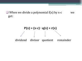
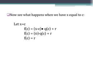
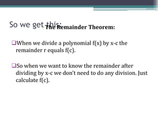
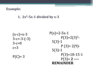
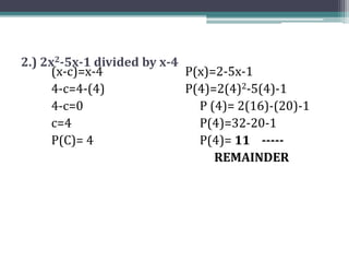
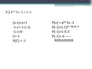
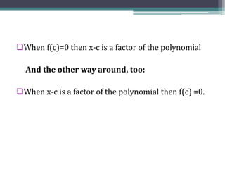
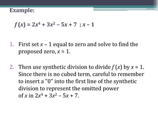
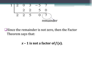
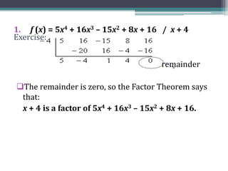
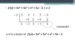
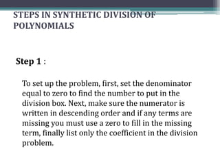
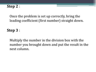
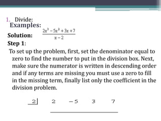
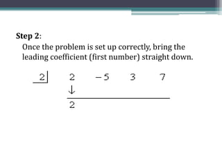
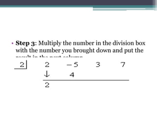
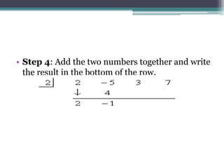
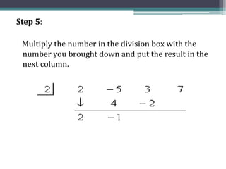
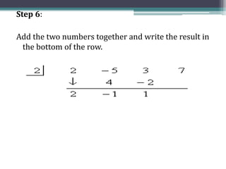
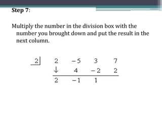
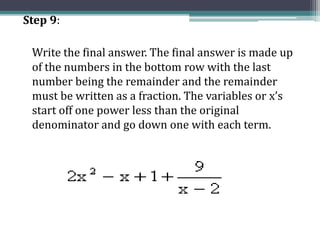
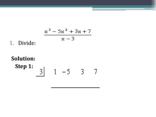
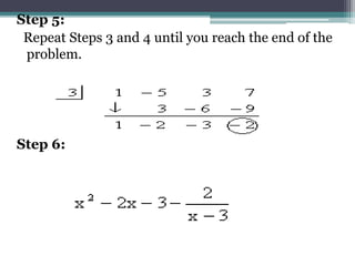
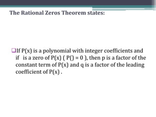
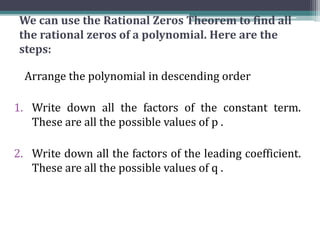
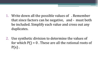
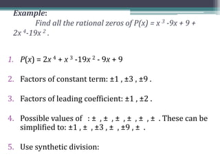
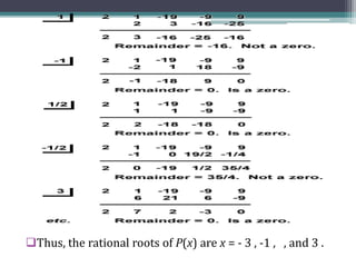
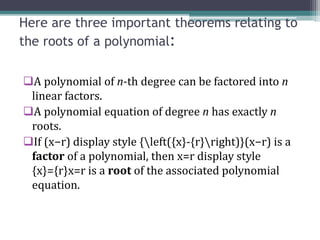
SlideShare a Scribd company logo
1 of 116
Finals’ Lessons in
ADVANCE ALGEBRA
a powerpoint compilation
THE REMAINDER THEOREM
 When we divide a polynomial f(x) by x-c we
get:
P(x) = (x-c) · q(x) + r(x)
dividend divisor quotient remainder
Now see what happens when we have x equal to c:
Let x=c
f(c) = (x-c)● q(c) + r
f(c) = (0)·q(c) + r
f(c) = r
So we get this:The Remainder Theorem:
When we divide a polynomial f(x) by x-c the
remainder r equals f(c).
So when we want to know the remainder after
dividing by x-c we don't need to do any division. Just
calculate f(c).
Example:
1. 2x2-5x-1 divided by x-3
(x-c)=x-3
3-c=-3-(-3)
3-c=0
c=3
P(C)= 3
P(x)=2-5x-1
P(3)=2(3)2-
5(3)-1
P (3)= 2(9)-
5(3)-1
P(3)=18-15-1
P(3)= 2 ----
REMAINDER
2.) 2x2-5x-1 divided by x-4
(x-c)=x-4
4-c=4-(4)
4-c=0
c=4
P(C)= 4
P(x)=2-5x-1
P(4)=2(4)2-5(4)-1
P (4)= 2(16)-(20)-1
P(4)=32-20-1
P(4)= 11 -----
REMAINDER
3.) x2+ 5x -3 / x+1
(x-c)=x+1
-1-c=-1-(-1)
-1-c=0
C=-1
P(C) = -1
P(x) = x2+ 5x -3
P(-1)=(-1)2 + 5(-1) -3
P(-1)=1-5-3
P(-1)=-6 -----
REMAINDER
THE FACTOR THEOREM
When f(c)=0 then x-c is a factor of the polynomial
And the other way around, too:
When x-c is a factor of the polynomial then f(c) =0.
Example:
f (x) = 2x4 + 3x2 – 5x + 7 ; x – 1
1. First set x – 1 equal to zero and solve to find the
proposed zero, x = 1.
2. Then use synthetic division to divide f (x) by x = 1.
Since there is no cubed term, careful to remember
to insert a "0" into the first line of the synthetic
division to represent the omitted power
of x in 2x4 + 3x2 – 5x + 7.
2 0 3 -5 7
2 2 5 0
remainder
Since the remainder is not zero, then the Factor
Theorem says that:
x – 1 is not a factor of f (x).
Exercise:
1. f (x) = 5x4 + 16x3 – 15x2 + 8x + 16 / x + 4
remainder
The remainder is zero, so the Factor Theorem says
that:
x + 4 is a factor of 5x4 + 16x3 – 15x2 + 8x + 16.
• f (x) = 3x4 + 5x3 + x2 + 5x – 2 / x+2
remainder
x+2 is a factor of f (x) = 3x4 + 5x3 + x2 + 5x – 2
SYNTHETIC DIVISION
Synthetic division is a shorthand method of dividing
polynomials where you divide the coefficients of the
polynomials, removing the variables and exponents.
It allows you to add throughout the process instead
of subtract, as you would do in traditional long
division.
STEPS IN SYNTHETIC DIVISION OF
POLYNOMIALS
Step 1 :
To set up the problem, first, set the denominator
equal to zero to find the number to put in the
division box. Next, make sure the numerator is
written in descending order and if any terms are
missing you must use a zero to fill in the missing
term, finally list only the coefficient in the division
problem.
Step 2 :
Once the problem is set up correctly, bring the
leading coefficient (first number) straight down.
Step 3 :
Multiply the number in the division box with the
number you brought down and put the result in the
next column.
Step 4 :
Add the two numbers together and write the result
in the bottom of the row.
Step 5 :
Repeat steps 3 and 4 until you reach the end of the
problem.
Step 6 :
Write the final answer. The final answer is made up
of the numbers in the bottom row with the last
number being the remainder and the remainder
must be written as a fraction. The variables or x’s
start off one power less than the original
denominator and go down one with each term.
Examples:
1. Divide:
Solution:
Step 1:
To set up the problem, first, set the denominator equal to
zero to find the number to put in the division box. Next,
make sure the numerator is written in descending order
and if any terms are missing you must use a zero to fill
in the missing term, finally list only the coefficient in the
division problem.
Step 2:
Once the problem is set up correctly, bring the
leading coefficient (first number) straight down.
• Step 3: Multiply the number in the division box
with the number you brought down and put the
result in the next column.
• Step 4: Add the two numbers together and write
the result in the bottom of the row.
Step 5:
Multiply the number in the division box with the
number you brought down and put the result in the
next column.
Step 6:
Add the two numbers together and write the result in
the bottom of the row.
Step 7:
Multiply the number in the division box with the
number you brought down and put the result in the
next column.
Step 8:
Add the two numbers together and write the result
in the bottom of the row.
Step 9:
Write the final answer. The final answer is made up
of the numbers in the bottom row with the last
number being the remainder and the remainder
must be written as a fraction. The variables or x’s
start off one power less than the original
denominator and go down one with each term.
1. Divide:
Solution:
Step 1:
Step 2:
Step 3:
Step 4:
Step 5:
Repeat Steps 3 and 4 until you reach the end of the
problem.
Step 6:
RATIONAL ZEROS OF POLYNOMIAL
FUNCTION
The Rational Zeros Theorem states:
If P(x) is a polynomial with integer coefficients and
if is a zero of P(x) ( P() = 0 ), then p is a factor of the
constant term of P(x) and q is a factor of the leading
coefficient of P(x) .
We can use the Rational Zeros Theorem to find all
the rational zeros of a polynomial. Here are the
steps:
Arrange the polynomial in descending order
1. Write down all the factors of the constant term.
These are all the possible values of p .
2. Write down all the factors of the leading coefficient.
These are all the possible values of q .
1. Write down all the possible values of . Remember
that since factors can be negative, and - must both
be included. Simplify each value and cross out any
duplicates.
2. Use synthetic division to determine the values of
for which P() = 0 . These are all the rational roots of
P(x) .
Example:
Find all the rational zeros of P(x) = x 3 -9x + 9 +
2x 4-19x 2 .
1. P(x) = 2x 4 + x 3 -19x 2 - 9x + 9
2. Factors of constant term: ±1 , ±3 , ±9 .
3. Factors of leading coefficient: ±1 , ±2 .
4. Possible values of : ± , ± , ± , ± , ± , ± . These can be
simplified to: ±1 , ± , ±3 , ± , ±9 , ± .
5. Use synthetic division:
Thus, the rational roots of P(x) are x = - 3 , -1 , , and 3 .
REAL ROOTS OF A POLYNOMIAL EQUATION
Here are three important theorems relating to
the roots of a polynomial:
A polynomial of n-th degree can be factored into n
linear factors.
A polynomial equation of degree n has exactly n
roots.
If (x−r) display style {left({x}-{r}right)}(x−r) is a
factor of a polynomial, then x=r display style
{x}={r}x=r is a root of the associated polynomial
equation.
The cubic polynomial f(x) = 4x3 − 3x2 − 25x −
6 has degree 3 (since the highest power of x that
appears is 3. This polynomial can be factored
and written as
4x3 − 3x2 − 25x − 6 = (x − 3)(4x + 1)(x +
2)
So we see that a 3rd degree polynomial has 3
roots.
 The associated polynomial equation is formed by
setting the polynomial equal to zero:
f(x) = 4x3 − 3x2 − 25x − 6 = 0
 In factored form, this is:
(x−3)(4x+1)(x+2)=0.
In this example, all 3 roots of our polynomial
equation of degree 3 are real.
 Since (x−3) is a factor, then x=3 is a root.
 Since (4x+1is a factor, then x=−​4​​1​​ is a root.
 Since (x+2) is a factor, then x=−2 is a root.
Solving Polynomials
The first step is to apply the Rational Roots Test to the
polynomial to get a list of values that might possibly be
solutions to the polynomial equation. You can follow this
up with an application of Descartes' Rule of Signs, if you
like, to narrow down which possible zeroes might be best
to check.
Of course, if you've got a graphing calculator, it's a good
idea to do a quick graph, since x-intercepts of the graph
are the same as zeroes of the equation.
Seeing where the graph looks like it crosses the axis can
quickly narrow down your list of possible zeroes.
Once you've found a value you want to test, you use
synthetic division to see if you can get a zero remainder.
If you get a zero remainder, you've not only found a zero,
but you've also reduced your polynomial by one degree.
 Remember that synthetic division is, among other
things, division, so checking if x = a is a solution is the
same as dividing out the linear factor x – a.
This means that you should not return to the original
polynomial for your next computation (for finding the
other zeroes); you should instead work with the output
of the synthetic division.
EXPONENTIAL FUNCTIONS AND THEIR
GRAPH
Let’s start off this section with the definition of an
exponential function.
If b is any number such that
and
then an exponential function is a function in the
form,
where b is called the base and x can be any
real number.
Notice that the x is now in the exponent and the
base is a fixed number. This is exactly the opposite
from what we’ve seen to this point. To this point the
base has been the variable, x in most cases, and the
exponent was a fixed number. However, despite
these differences these functions evaluate in exactly
the same way as those that we are used to. We will
see some examples of exponential functions shortly.
Before we get too far into this section we should
address the restrictions on b. We avoid one and zero
because in this case the function would be,
and these are constant functions and won’t have
many of the same properties that general
exponential functions have.
Next, we avoid negative numbers so that we don’t
get any complex values out of the function
evaluation. For instance if we allowed the
function would be,
and as you can see there are some function
evaluations that will give complex numbers. We
only want real numbers to arise from function
evaluation and so to make sure of this we require
that b not be a negative number.
Now, let’s take a look at a couple of graphs. We will
be able to get most of the properties of exponential
functions from these graphs.
Example 1: Sketch the graph of and
and
on the same axis system.
Solution
Okay, since we don’t have any knowledge on
what these graphs look like we’re going to have to
pick some values of x and do some function
evaluations. Function evaluation with exponential
functions works in exactly the same manner that all
function evaluation has worked to this
point. Whatever is in the parenthesis on the left we
substitute into all the x’s on the right side.
Here are some evaluations for these two functions,
x
-2
-1
0
1
2
Here is the sketch of the two graphs.
Note as well that we could have written in
the following way,
--- Sometimes we’ll see this kind of exponential
function and so it’s important to be able to go
between these two forms.
Properties of Exponential Functions.
1. The graph of will always contain the point .
Or put another way, regardless of the value of b.
2. For every possible b . Note that this implies
that .
3. If then the graph of will decrease as we
move from left to right. Check out the graph
of above for verification of this property.
4. If then the graph of will increase as we
move from left to right. Check out the graph
of above for verification of this property.
5. If then .
--- All of these properties except the final one can be
verified easily from the graphs in the first
example. We will hold off discussing the final
property for a couple of sections where we will
actually be using it.
Example 2
Sketch the graph of
Solution
Let’s first build up a table of values for this function.
• To get these evaluation you will need to use a
calculator. In fact, that is part of the point of this
example. Make sure that you can run your
calculator and verify these numbers.
x -2 -1 0 1 2
f(x) 0.135 0.3679 1 2.178 7.389
Here is a sketch of this graph.
Notice that this is an increasing graph as we should
expect since
There is one final example that we need to work
before moving onto the next section. This example
is more about the evaluation process for
exponential functions than the graphing
process. We need to be very careful with the
evaluation of exponential functions.
Example 3
Sketch the graph of
Solution
Here is a quick table of values for this function.
Now, as we stated above this example was more
about the evaluation process than the graph so
let’s go through the first one to make sure that you
can do these.
x -1 0 1 2 3
g(x) 32.945… 9.951…. 1 -2.161… -3.323…
 Notice that when evaluating exponential
functions we first need to actually do the
exponentiation before we multiply by any
coefficients (5 in this case). Also, we used only 3
decimal places here since we are only graphing. In
many applications we will want to use far more
decimal places in these computations.
Here is a sketch of the graph.
Notice that this graph violates all the properties
we listed above. That is okay. Those properties
are only valid for functions in the
form or . We’ve got a lot more
going on in this function and so the properties, as
written above, won’t hold for this function.
Logarithmic Functions & Their Graphs
For x  0 and 0  a  1,
y = loga x if and only if x = a y.
The function given by f (x) = loga x is called the
logarithmic function with base a.
Every logarithmic equation has an equivalent
exponential form:
y = loga x is equivalent to x = a y
A logarithm is an exponent!
 A logarithmic function is the inverse function of an
exponential function.
Exponential function: y = ax
Logarithmic function: y = logax is equivalent to x = ay
Examples:
Write the equivalent exponential equation
and solve for y.
Logarithmic
Functions & Their
Graphs
Equivalent
Exponential
Equation
Solution
y = log216
y = log2( )
y = log416
y = log51
16 = 2y
= 2 y
16 = 4y
1 = 5 y
16 = 24  y = 4
= 2-1 y = –1
16 = 42  y = 2
1 = 50  y = 0
Copyright © by Houghton Mifflin Company, Inc. All rights reserved. 5
Properties of Logarithms
Examples: Solve for x: log6 6 = x
log6 6 = 1 property 2 x = 1
Simplify: log3 35
log3 35 = 5 property 3
Simplify: 7log
7
9
7log
7
9 = 9 property 3
Properties of Logarithms
1. loga 1 = 0 since a0 = 1.
2. loga a = 1 since a1 = a.
4. If loga x = loga y, then x = y. one-to-one property
3. loga ax = x and alogax = x inverse property
Copyright © by Houghton Mifflin Company, Inc. All rights reserved. 7
Example: Graph the common logarithm function f(x) = log10 x.
by calculator
1
10
10.6020.3010–1–2f(x) = log10 x
10421x 1
100
y
x
5
–5
f(x) = log10 x
x = 0
vertical
asymptote
(0, 1) x-intercept
Copyright © by Houghton Mifflin Company, Inc. All rights reserved. 8
The graphs of logarithmic functions are similar for different
values of a.
f(x) = loga x (a  1)
3. x-intercept (1, 0)
5. increasing
6. continuous
7. one-to-one
8. reflection of y = ax in y = x
1. domain ),0( 
2. range ),( 
4. vertical asymptote
 
)(0as0 xfxx
Graph of f(x) = loga x (a  1)
x
y y = x
y = log2 x
y = ax
domain
range
y-axis
vertical
asymptote
x-intercept
(1, 0)
Copyright © by Houghton Mifflin Company, Inc. All rights reserved. 9
The function defined by
f(x) = loge x = ln x
is called the natural
logarithm function.
Use a calculator to evaluate: ln 3, ln –2, ln 100
ln 3
ln –2
ln 100
Function Value Keystrokes Display
LN 3 ENTER 1.0986122
ERRORLN –2 ENTER
LN 100 ENTER 4.6051701
y = ln x
(x  0, e 2.718281)
y
x
5
–5
y = ln x is equivalent to ey = x
PROPERTIES OF LOGARITHMS
loga 1 = 0 because a0 = 1
No matter what the base is, as long as it is legal, the
log of 1 is always 0. That's because logarithmic
curves always pass through (1,0)
loga a = 1 because a1 = a
Any value raised to the first power is that same
value.
loga ax = x
The log base a of x and a to the x power are inverse
functions. Whenever inverse functions are applied
to each other, they inverse out, and you're left with
the argument, in this case, x.
loga x = loga y implies that x = y
If two logs with the same base are equal, then the
arguments must be equal.
loga x = logb x implies that a = b
If two logarithms with the same argument are equal,
then the bases must be equal.
LOGARITHMS
When we are given the base 2, for example, and exponent
3, then we can evaluate 23.
23 = 8.
Inversely, if we are given the base 2 and its power 8 – (2?=
8) then what is the exponent that will produce 8?
That exponent is called a logarithm. We call the exponent
3 the logarithm of 8 with base 2.
We write 3 = log28
We write the base 2 as a subscript.
3 is the exponent to which 2 must be raised to produce 8.
A logarithm is an exponent.
Since 104 = 10,000 then log1010,000 = 4.
"The logarithm of 10,000 with base 10 is 4."
4 is the exponent to which 10 must be raised to
produce 10,000.
"104 = 10,000" is called the exponential form.
"log1010,000 = 4" is called the logarithmic form.
logbx = n means bn = x.
Example 1.
Write in exponential form: log232 = 5.
Answer. 25 = 32.
Example 2.
Write in logarithmic form: 4−2 = 1
16
Answer. log4 1 = −2.
16
THE LAW OF LOGARITHMS:
The first law of logarithms
--- relates multiplication to addition and states that
the logarithm of a product of two terms A and B is
the sum of the logarithms of those terms so that:
logAB logAlogB
--- This law is true for any base of logarithm so
long as you use the same base throughout a
calculation. You could re-write law 1 in base a as:
ABAB as a log loglog
You should remember that, because of the equals
sign, this law also works from right-to-left and so
can be used to combine logarithms of the same base
that are added together. When quoting this law you
should try to say it in full as it is often
misremembered as “the log of A plus B”. If you make
the effort to quote it in full then this (very common)
error can be avoided: There is no law of logarithms
which relates to logAB.
Example:
Rewrite log15 in terms of log3 and log5. As 15 
35 you can use law 1 with A  3 and B  5 So, for any
base:
log(15)  log35 log3log5
Example: Express lnxln(3) as a single logarithm.
As lnxln(3) is the sum of two logarithms both in base e
(natural logarithm), you can use law 1 to show that:
lnxln3ln3 xln3x
Where the answer also has to be a natural logarithm
 The second law of logarithms
--- In the same way that law 1 relates multiplication to
addition, law 2 relates division to subtraction. The law
states that the logarithm of a quotient of two terms A
and B is the logarithm of the numerator minus the
logarithm of the denominator so that:
log)= log (A)- log(B)
 Similar to law 1, the equals sign means that this
law also works from right-to-left. When quoting this
law you should try to say it in full as it is often
misremembered as “the log of A minus B”. If you
make the effort to quote it in full then this (very
common) error can be avoided: There is no law of
logarithms which relates to logAB or B A log log .
Example:
 Express log () in terms of logx and log4.
This is a logarithm of a fraction with A x and B  4 so
you can use law 2 to show that, for any base:
Log= log (x)- log (4)
The third law of logarithms
--- relates exponentiation (raising to a power) to
multiplication and states that the logarithm of A
raised to the power of n is n multiplied by the
logarithm of A:
log(An) = nlog(A)
The logarithm of A divided by B is the logarithm of
A minus the logarithm of B As with the other two
laws, you need to use the same base throughout a
calculation:
loga(An) = nloga(A)
This law also works from right-to-left and can be
used to change a number that is multiplied by a
logarithm into exponentiation; law 3 is often
thought of as the most important because of this.
It is especially useful when changing relationships
described by curves into straight lines. The final
section of this guide shows you how to change an
exponential function into a straight line.
Example:
 Calculate log3(9).
This may not seem like a question where
you can use law 3. However, as 9 = 32 you can
use law 3 with A  3 and n 2 to find that:
log3(9) = log3 (32) = 2log3(3)
SOLVING EXPONENTIAL EQUATIONS
An exponential equation is one in which a variable
occurs in the exponent.
An exponential equation in which each side can be
expressed in
terms of the same base can be solved using the
property:
If the bases are the same, set the exponents equal.
Rule:
To solve an exponential equation, take the log of both sides,
and solve for the variable.
Example 1:
Solve for x in the equation
Solution:
Step 1:
Take the natural log of both sides:
Step 2:
Simplify the left side of the above equation
using Logarithmic Rule 3:
Step 3:
Simplify the left side of the above equation:
Since Ln(e)=1, the equation reads
Ln(80) is the exact answer
and x=4.38202663467 is an approximate answer
because we have rounded the value of Ln(80)..
Check:
Check your answer in the original equation.
Example 2:
Solve for x in the equation
Solution:
Step 1:
Isolate the exponential term before you take the
common log of both sides. Therefore, add 8 to both
sides:
Step 2:
Take the common log of both sides:
Step 3:
Simplify the left side of the above equation using
Logarithmic Rule 3:
Step 4:
Simplify the left side of the above equation: Since
Log(10) = 1, the above equation can be written
Step 5:
Subtract 5 from both sides of the above
equation:
is the exact answer. x = -3.16749108729 is an
approximate answer..
Check:
Check your answer in the original equation
SOLVING LOGARITHMIC EQUATIONS
• Logarithmic equations contain logarithmic
expressions and constants. A logarithm is another
way to write an exponent and is defined
by if and only if . .
• When one side of the equation contains a single
logarithm and the other side contains a constant,
the equation can be solved by rewriting the
equation as an equivalent exponential equation
using the definition of logarithm from above.
Rule:
To solve a logarithmic equation, rewrite the equation in
exponential form and solve for the variable.
Example 1:
Solve for x in the equation Ln(x)=8
Solution:
Step 1:
Let both sides be exponents of the base e. The
equation Ln(x)=8 can be rewritten .
• Step 2: By now you should know that when the base
of the exponent and the base of the logarithm are the
same, the left side can be written x. The
equation can now be written .
Step 3:
The exact answer is
and the approximate answer is
Example 2:
Solve for x in the equation
Answer:
is the exact answer
and x=104.142857143 is an approximate answer.
Solution:
Step 1: Since you cannot take the log of a negative
number, we have to restrict the domain so that 7x >0
or x > 0.
Step 2: Isolate the Log term in the original equation by
subtracting 4 from each side of the equation:
Step 3:
Convert the above logarithmic equation to an
exponential equation with base 3 and exponent 6:
Step 4: Divide both sides of the above equation
by 7:
is the exact answer and is an approximate
answer.
Check:
Let's substitute the approximate value in the
answer and determine whether the left side of the
equation equals the right side of the equation after
the substitution. Remember we rounded the
number and the answer is only a close
approximation, so the left and right side of the
equation will most likely be very close but not equal;
it depends on the number of decimals were rounded
in your answer
Or
EXPONENTIAL EQUATION AND
LOGARITHMIC MODEL
An exponential equation is one in which a variable
occurs in the exponent.
An exponential equation in which each side can be
expressed in
terms of the same base can be solved using the
property:
If the bases are the same, set the exponents equal
Examples:Solve for x. Answer
1.
Since the bases are the same, set the
exponents equal to one another:
2x + 1 = 3x - 2
3 = x
2.
27 can be expressed as a power of 3:
2x - 1 = 3x
-1 = x
3.
25 can be expressed as a power of 5:
3x - 8 = 4x
-8 = x
Exponential Growth
FUNCTIONy = C ekt, k > 0
Features
Asymptotic to y = 0 to left
Passes through (0,C)
C is the initial value
Increases without bound to right
Exponential Decay (decreasing form)
FUNCTIONy = C e-kt, k > 0
Features
Asymptotic to y = 0 to right
Passes through (0,C)
C is the initial value
Decreasing, but bounded below by y=0
LOGARITHMIC MODEL
FUNCTIONy = a + b ln x
Features
Increases without bound to right
Passes through (1,a),
Very rapid growth, followed by slower growth,
Common log will grow slower than natural log
b controls the rate of growth
The logarithmic model has a period of rapid
increase, followed by a period where the growth
slows, but the growth continues to increase without
bound.
 This makes the model inappropriate where there
needs to be an upper bound.
The main difference between this model and the
exponential growth model is that the exponential
growth model begins slowly and then increases very
rapidly as time increases.
Submitted by:
Allado, Swedenia
Artizona, Anamae
Bolivar, Ma. Cris
Annabelle
Callocallo, April
Mae
Gabilagon, Liezl
Lerado, Aira
Grace
Matalubos, Lyra
Sorenio, Shiela
Mae
Tabuga, Natalie
T0rda, Marjocel
Submitted to:
Prof. Danilo Parreño
ADVANCE ALGEBRA

More Related Content

What's hot

Evaluating Algebraic Expressions
Evaluating Algebraic ExpressionsEvaluating Algebraic Expressions
Evaluating Algebraic Expressionsbizarregirl
 
Integers: Addition and Subtraction
Integers: Addition and SubtractionIntegers: Addition and Subtraction
Integers: Addition and SubtractionCarlo Luna
 
Solving Absolute Value Inequalities
Solving Absolute Value InequalitiesSolving Absolute Value Inequalities
Solving Absolute Value InequalitiesClayton Rainsberg
 
ALGEBRIC EXPRESSION 7.ppt
ALGEBRIC EXPRESSION 7.pptALGEBRIC EXPRESSION 7.ppt
ALGEBRIC EXPRESSION 7.pptInduSingh89
 
Algebraic expressions and equations
Algebraic expressions and equationsAlgebraic expressions and equations
Algebraic expressions and equationsChristian Costa
 
Factoring Trinomials
Factoring TrinomialsFactoring Trinomials
Factoring TrinomialsDon Simmons
 
Rounding Whole Numbers
Rounding Whole NumbersRounding Whole Numbers
Rounding Whole NumbersSteven Diaz
 
Rounding Numbers
Rounding NumbersRounding Numbers
Rounding Numbersmilenia86
 
1.2 Irrational Numbers ppt
1.2 Irrational Numbers ppt1.2 Irrational Numbers ppt
1.2 Irrational Numbers pptSandra Johnson
 
Expressions and equations
Expressions and equationsExpressions and equations
Expressions and equationsAron Dotson
 
5 6 laws of logarithms
5 6 laws of logarithms5 6 laws of logarithms
5 6 laws of logarithmshisema01
 
Sales,Percentage,discount,marked price (Math 6)
Sales,Percentage,discount,marked price (Math 6)Sales,Percentage,discount,marked price (Math 6)
Sales,Percentage,discount,marked price (Math 6)Sherwin Dulay
 
Square and square roots
Square and square rootsSquare and square roots
Square and square rootsJessica Garcia
 
Square root
Square rootSquare root
Square rootrryan80
 
Introduction to algebra
Introduction to algebraIntroduction to algebra
Introduction to algebraArvin Caya
 
Positive and negative numbers
Positive and negative numbersPositive and negative numbers
Positive and negative numberskkettler1
 

What's hot (20)

Evaluating Algebraic Expressions
Evaluating Algebraic ExpressionsEvaluating Algebraic Expressions
Evaluating Algebraic Expressions
 
Integers: Addition and Subtraction
Integers: Addition and SubtractionIntegers: Addition and Subtraction
Integers: Addition and Subtraction
 
Gemdas rule
Gemdas ruleGemdas rule
Gemdas rule
 
Solving Absolute Value Inequalities
Solving Absolute Value InequalitiesSolving Absolute Value Inequalities
Solving Absolute Value Inequalities
 
ALGEBRIC EXPRESSION 7.ppt
ALGEBRIC EXPRESSION 7.pptALGEBRIC EXPRESSION 7.ppt
ALGEBRIC EXPRESSION 7.ppt
 
Algebraic expressions and equations
Algebraic expressions and equationsAlgebraic expressions and equations
Algebraic expressions and equations
 
Factoring Trinomials
Factoring TrinomialsFactoring Trinomials
Factoring Trinomials
 
Decimal
DecimalDecimal
Decimal
 
Rounding Whole Numbers
Rounding Whole NumbersRounding Whole Numbers
Rounding Whole Numbers
 
Rounding Numbers
Rounding NumbersRounding Numbers
Rounding Numbers
 
1.2 Irrational Numbers ppt
1.2 Irrational Numbers ppt1.2 Irrational Numbers ppt
1.2 Irrational Numbers ppt
 
Expressions and equations
Expressions and equationsExpressions and equations
Expressions and equations
 
5 6 laws of logarithms
5 6 laws of logarithms5 6 laws of logarithms
5 6 laws of logarithms
 
Sales,Percentage,discount,marked price (Math 6)
Sales,Percentage,discount,marked price (Math 6)Sales,Percentage,discount,marked price (Math 6)
Sales,Percentage,discount,marked price (Math 6)
 
Maths amazing facts
Maths amazing factsMaths amazing facts
Maths amazing facts
 
Square and square roots
Square and square rootsSquare and square roots
Square and square roots
 
Square root
Square rootSquare root
Square root
 
Introduction to algebra
Introduction to algebraIntroduction to algebra
Introduction to algebra
 
Integers
IntegersIntegers
Integers
 
Positive and negative numbers
Positive and negative numbersPositive and negative numbers
Positive and negative numbers
 

Viewers also liked

Pre Calculus notes 4 1 Exponential Functions
Pre Calculus notes 4 1 Exponential FunctionsPre Calculus notes 4 1 Exponential Functions
Pre Calculus notes 4 1 Exponential Functionsmsventrella
 
Linear Equation With One Variable
Linear Equation With One VariableLinear Equation With One Variable
Linear Equation With One VariableMoerti Utami
 
Math Sample Age Problem
Math Sample Age ProblemMath Sample Age Problem
Math Sample Age Problemliyanoo
 
Linear Equation In one variable class 7
 Linear Equation In one variable class 7 Linear Equation In one variable class 7
Linear Equation In one variable class 7Poulami Choudhury
 
Solve Math Word Problems
Solve Math Word ProblemsSolve Math Word Problems
Solve Math Word ProblemsAllAboutHSCurr
 
Algebra "Age Problem"
Algebra "Age Problem"Algebra "Age Problem"
Algebra "Age Problem"guestc71130
 
Linear Equations and Inequalities in One Variable
Linear Equations and Inequalities in One VariableLinear Equations and Inequalities in One Variable
Linear Equations and Inequalities in One Variablemisey_margarette
 

Viewers also liked (15)

My powerpoint
My powerpointMy powerpoint
My powerpoint
 
Facebook demographics power point
Facebook demographics power pointFacebook demographics power point
Facebook demographics power point
 
Pre Calculus notes 4 1 Exponential Functions
Pre Calculus notes 4 1 Exponential FunctionsPre Calculus notes 4 1 Exponential Functions
Pre Calculus notes 4 1 Exponential Functions
 
Advance algebra
Advance algebraAdvance algebra
Advance algebra
 
Exponentials
ExponentialsExponentials
Exponentials
 
Word Problems Linear
Word Problems LinearWord Problems Linear
Word Problems Linear
 
Linear Equation With One Variable
Linear Equation With One VariableLinear Equation With One Variable
Linear Equation With One Variable
 
Math Sample Age Problem
Math Sample Age ProblemMath Sample Age Problem
Math Sample Age Problem
 
Word Problems
Word ProblemsWord Problems
Word Problems
 
Linear Equation In one variable class 7
 Linear Equation In one variable class 7 Linear Equation In one variable class 7
Linear Equation In one variable class 7
 
Solve Math Word Problems
Solve Math Word ProblemsSolve Math Word Problems
Solve Math Word Problems
 
Algebra "Age Problem"
Algebra "Age Problem"Algebra "Age Problem"
Algebra "Age Problem"
 
Linear Equations and Inequalities in One Variable
Linear Equations and Inequalities in One VariableLinear Equations and Inequalities in One Variable
Linear Equations and Inequalities in One Variable
 
linear equation
linear equationlinear equation
linear equation
 
Solving Word problems
Solving Word problemsSolving Word problems
Solving Word problems
 

Similar to Advance algebra

Module 3 polynomial functions
Module 3   polynomial functionsModule 3   polynomial functions
Module 3 polynomial functionsdionesioable
 
Presentación grupo 551108 30
Presentación grupo 551108 30Presentación grupo 551108 30
Presentación grupo 551108 30njhernandez19
 
Maths notes for 4038 and 4016 paper
Maths notes for 4038 and 4016 paperMaths notes for 4038 and 4016 paper
Maths notes for 4038 and 4016 paperFabian Hkb
 
6.3 evaluating-and-graphing-polynomila-functions
6.3 evaluating-and-graphing-polynomila-functions6.3 evaluating-and-graphing-polynomila-functions
6.3 evaluating-and-graphing-polynomila-functionsmorrobea
 
6.3 evaluating-and-graphing-polynomila-functions
6.3 evaluating-and-graphing-polynomila-functions6.3 evaluating-and-graphing-polynomila-functions
6.3 evaluating-and-graphing-polynomila-functionsmorrobea
 
3.4 Polynomial Functions and Their Graphs
3.4 Polynomial Functions and Their Graphs3.4 Polynomial Functions and Their Graphs
3.4 Polynomial Functions and Their Graphssmiller5
 
May 28, 2014
May 28, 2014May 28, 2014
May 28, 2014khyps13
 
Polynomial Function and Synthetic Division
Polynomial Function and Synthetic DivisionPolynomial Function and Synthetic Division
Polynomial Function and Synthetic DivisionAleczQ1414
 
3.4 Polynomial Functions and Their Graphs
3.4 Polynomial Functions and Their Graphs3.4 Polynomial Functions and Their Graphs
3.4 Polynomial Functions and Their Graphssmiller5
 
Chapter 5 Polynomials
Chapter 5 PolynomialsChapter 5 Polynomials
Chapter 5 PolynomialsReema
 
Module 2 Lesson 2 Notes
Module 2 Lesson 2 NotesModule 2 Lesson 2 Notes
Module 2 Lesson 2 Notestoni dimella
 
0.1.basic arith.&set
0.1.basic arith.&set0.1.basic arith.&set
0.1.basic arith.&setm2699
 
Appendex b
Appendex bAppendex b
Appendex bswavicky
 

Similar to Advance algebra (20)

Module 3 polynomial functions
Module 3   polynomial functionsModule 3   polynomial functions
Module 3 polynomial functions
 
Ppt on polynomial
Ppt on polynomial Ppt on polynomial
Ppt on polynomial
 
Rational_Functions.pptx
Rational_Functions.pptxRational_Functions.pptx
Rational_Functions.pptx
 
Presentación grupo 551108 30
Presentación grupo 551108 30Presentación grupo 551108 30
Presentación grupo 551108 30
 
Maths notes for 4038 and 4016 paper
Maths notes for 4038 and 4016 paperMaths notes for 4038 and 4016 paper
Maths notes for 4038 and 4016 paper
 
6.3 evaluating-and-graphing-polynomila-functions
6.3 evaluating-and-graphing-polynomila-functions6.3 evaluating-and-graphing-polynomila-functions
6.3 evaluating-and-graphing-polynomila-functions
 
6.3 evaluating-and-graphing-polynomila-functions
6.3 evaluating-and-graphing-polynomila-functions6.3 evaluating-and-graphing-polynomila-functions
6.3 evaluating-and-graphing-polynomila-functions
 
3.4 Polynomial Functions and Their Graphs
3.4 Polynomial Functions and Their Graphs3.4 Polynomial Functions and Their Graphs
3.4 Polynomial Functions and Their Graphs
 
May 28, 2014
May 28, 2014May 28, 2014
May 28, 2014
 
Polynomial Function and Synthetic Division
Polynomial Function and Synthetic DivisionPolynomial Function and Synthetic Division
Polynomial Function and Synthetic Division
 
3.4 Polynomial Functions and Their Graphs
3.4 Polynomial Functions and Their Graphs3.4 Polynomial Functions and Their Graphs
3.4 Polynomial Functions and Their Graphs
 
Polynomials lecture
Polynomials lecturePolynomials lecture
Polynomials lecture
 
Chapter 5 Polynomials
Chapter 5 PolynomialsChapter 5 Polynomials
Chapter 5 Polynomials
 
Module 2 Lesson 2 Notes
Module 2 Lesson 2 NotesModule 2 Lesson 2 Notes
Module 2 Lesson 2 Notes
 
OPERATIONS RESEARCH
OPERATIONS RESEARCHOPERATIONS RESEARCH
OPERATIONS RESEARCH
 
0.1.basic arith.&set
0.1.basic arith.&set0.1.basic arith.&set
0.1.basic arith.&set
 
Polynomial equations
Polynomial equationsPolynomial equations
Polynomial equations
 
BP106RMT.pdf
BP106RMT.pdfBP106RMT.pdf
BP106RMT.pdf
 
Appendex b
Appendex bAppendex b
Appendex b
 
Division of polynomials
Division of polynomialsDivision of polynomials
Division of polynomials
 

Recently uploaded

Employee wellbeing at the workplace.pptx
Employee wellbeing at the workplace.pptxEmployee wellbeing at the workplace.pptx
Employee wellbeing at the workplace.pptxNirmalaLoungPoorunde1
 
Concept of Vouching. B.Com(Hons) /B.Compdf
Concept of Vouching. B.Com(Hons) /B.CompdfConcept of Vouching. B.Com(Hons) /B.Compdf
Concept of Vouching. B.Com(Hons) /B.CompdfUmakantAnnand
 
Introduction to ArtificiaI Intelligence in Higher Education
Introduction to ArtificiaI Intelligence in Higher EducationIntroduction to ArtificiaI Intelligence in Higher Education
Introduction to ArtificiaI Intelligence in Higher Educationpboyjonauth
 
How to Make a Pirate ship Primary Education.pptx
How to Make a Pirate ship Primary Education.pptxHow to Make a Pirate ship Primary Education.pptx
How to Make a Pirate ship Primary Education.pptxmanuelaromero2013
 
Contemporary philippine arts from the regions_PPT_Module_12 [Autosaved] (1).pptx
Contemporary philippine arts from the regions_PPT_Module_12 [Autosaved] (1).pptxContemporary philippine arts from the regions_PPT_Module_12 [Autosaved] (1).pptx
Contemporary philippine arts from the regions_PPT_Module_12 [Autosaved] (1).pptxRoyAbrique
 
Mastering the Unannounced Regulatory Inspection
Mastering the Unannounced Regulatory InspectionMastering the Unannounced Regulatory Inspection
Mastering the Unannounced Regulatory InspectionSafetyChain Software
 
Hybridoma Technology ( Production , Purification , and Application )
Hybridoma Technology  ( Production , Purification , and Application  ) Hybridoma Technology  ( Production , Purification , and Application  )
Hybridoma Technology ( Production , Purification , and Application ) Sakshi Ghasle
 
Organic Name Reactions for the students and aspirants of Chemistry12th.pptx
Organic Name Reactions  for the students and aspirants of Chemistry12th.pptxOrganic Name Reactions  for the students and aspirants of Chemistry12th.pptx
Organic Name Reactions for the students and aspirants of Chemistry12th.pptxVS Mahajan Coaching Centre
 
KSHARA STURA .pptx---KSHARA KARMA THERAPY (CAUSTIC THERAPY)————IMP.OF KSHARA ...
KSHARA STURA .pptx---KSHARA KARMA THERAPY (CAUSTIC THERAPY)————IMP.OF KSHARA ...KSHARA STURA .pptx---KSHARA KARMA THERAPY (CAUSTIC THERAPY)————IMP.OF KSHARA ...
KSHARA STURA .pptx---KSHARA KARMA THERAPY (CAUSTIC THERAPY)————IMP.OF KSHARA ...M56BOOKSTORE PRODUCT/SERVICE
 
18-04-UA_REPORT_MEDIALITERAСY_INDEX-DM_23-1-final-eng.pdf
18-04-UA_REPORT_MEDIALITERAСY_INDEX-DM_23-1-final-eng.pdf18-04-UA_REPORT_MEDIALITERAСY_INDEX-DM_23-1-final-eng.pdf
18-04-UA_REPORT_MEDIALITERAСY_INDEX-DM_23-1-final-eng.pdfssuser54595a
 
Science 7 - LAND and SEA BREEZE and its Characteristics
Science 7 - LAND and SEA BREEZE and its CharacteristicsScience 7 - LAND and SEA BREEZE and its Characteristics
Science 7 - LAND and SEA BREEZE and its CharacteristicsKarinaGenton
 
SOCIAL AND HISTORICAL CONTEXT - LFTVD.pptx
SOCIAL AND HISTORICAL CONTEXT - LFTVD.pptxSOCIAL AND HISTORICAL CONTEXT - LFTVD.pptx
SOCIAL AND HISTORICAL CONTEXT - LFTVD.pptxiammrhaywood
 
CARE OF CHILD IN INCUBATOR..........pptx
CARE OF CHILD IN INCUBATOR..........pptxCARE OF CHILD IN INCUBATOR..........pptx
CARE OF CHILD IN INCUBATOR..........pptxGaneshChakor2
 
Sanyam Choudhary Chemistry practical.pdf
Sanyam Choudhary Chemistry practical.pdfSanyam Choudhary Chemistry practical.pdf
Sanyam Choudhary Chemistry practical.pdfsanyamsingh5019
 
Solving Puzzles Benefits Everyone (English).pptx
Solving Puzzles Benefits Everyone (English).pptxSolving Puzzles Benefits Everyone (English).pptx
Solving Puzzles Benefits Everyone (English).pptxOH TEIK BIN
 
mini mental status format.docx
mini    mental       status     format.docxmini    mental       status     format.docx
mini mental status format.docxPoojaSen20
 
Separation of Lanthanides/ Lanthanides and Actinides
Separation of Lanthanides/ Lanthanides and ActinidesSeparation of Lanthanides/ Lanthanides and Actinides
Separation of Lanthanides/ Lanthanides and ActinidesFatimaKhan178732
 
Accessible design: Minimum effort, maximum impact
Accessible design: Minimum effort, maximum impactAccessible design: Minimum effort, maximum impact
Accessible design: Minimum effort, maximum impactdawncurless
 
POINT- BIOCHEMISTRY SEM 2 ENZYMES UNIT 5.pptx
POINT- BIOCHEMISTRY SEM 2 ENZYMES UNIT 5.pptxPOINT- BIOCHEMISTRY SEM 2 ENZYMES UNIT 5.pptx
POINT- BIOCHEMISTRY SEM 2 ENZYMES UNIT 5.pptxSayali Powar
 

Recently uploaded (20)

Employee wellbeing at the workplace.pptx
Employee wellbeing at the workplace.pptxEmployee wellbeing at the workplace.pptx
Employee wellbeing at the workplace.pptx
 
Concept of Vouching. B.Com(Hons) /B.Compdf
Concept of Vouching. B.Com(Hons) /B.CompdfConcept of Vouching. B.Com(Hons) /B.Compdf
Concept of Vouching. B.Com(Hons) /B.Compdf
 
Introduction to ArtificiaI Intelligence in Higher Education
Introduction to ArtificiaI Intelligence in Higher EducationIntroduction to ArtificiaI Intelligence in Higher Education
Introduction to ArtificiaI Intelligence in Higher Education
 
How to Make a Pirate ship Primary Education.pptx
How to Make a Pirate ship Primary Education.pptxHow to Make a Pirate ship Primary Education.pptx
How to Make a Pirate ship Primary Education.pptx
 
Contemporary philippine arts from the regions_PPT_Module_12 [Autosaved] (1).pptx
Contemporary philippine arts from the regions_PPT_Module_12 [Autosaved] (1).pptxContemporary philippine arts from the regions_PPT_Module_12 [Autosaved] (1).pptx
Contemporary philippine arts from the regions_PPT_Module_12 [Autosaved] (1).pptx
 
Mastering the Unannounced Regulatory Inspection
Mastering the Unannounced Regulatory InspectionMastering the Unannounced Regulatory Inspection
Mastering the Unannounced Regulatory Inspection
 
Hybridoma Technology ( Production , Purification , and Application )
Hybridoma Technology  ( Production , Purification , and Application  ) Hybridoma Technology  ( Production , Purification , and Application  )
Hybridoma Technology ( Production , Purification , and Application )
 
Organic Name Reactions for the students and aspirants of Chemistry12th.pptx
Organic Name Reactions  for the students and aspirants of Chemistry12th.pptxOrganic Name Reactions  for the students and aspirants of Chemistry12th.pptx
Organic Name Reactions for the students and aspirants of Chemistry12th.pptx
 
KSHARA STURA .pptx---KSHARA KARMA THERAPY (CAUSTIC THERAPY)————IMP.OF KSHARA ...
KSHARA STURA .pptx---KSHARA KARMA THERAPY (CAUSTIC THERAPY)————IMP.OF KSHARA ...KSHARA STURA .pptx---KSHARA KARMA THERAPY (CAUSTIC THERAPY)————IMP.OF KSHARA ...
KSHARA STURA .pptx---KSHARA KARMA THERAPY (CAUSTIC THERAPY)————IMP.OF KSHARA ...
 
18-04-UA_REPORT_MEDIALITERAСY_INDEX-DM_23-1-final-eng.pdf
18-04-UA_REPORT_MEDIALITERAСY_INDEX-DM_23-1-final-eng.pdf18-04-UA_REPORT_MEDIALITERAСY_INDEX-DM_23-1-final-eng.pdf
18-04-UA_REPORT_MEDIALITERAСY_INDEX-DM_23-1-final-eng.pdf
 
Science 7 - LAND and SEA BREEZE and its Characteristics
Science 7 - LAND and SEA BREEZE and its CharacteristicsScience 7 - LAND and SEA BREEZE and its Characteristics
Science 7 - LAND and SEA BREEZE and its Characteristics
 
SOCIAL AND HISTORICAL CONTEXT - LFTVD.pptx
SOCIAL AND HISTORICAL CONTEXT - LFTVD.pptxSOCIAL AND HISTORICAL CONTEXT - LFTVD.pptx
SOCIAL AND HISTORICAL CONTEXT - LFTVD.pptx
 
CARE OF CHILD IN INCUBATOR..........pptx
CARE OF CHILD IN INCUBATOR..........pptxCARE OF CHILD IN INCUBATOR..........pptx
CARE OF CHILD IN INCUBATOR..........pptx
 
Sanyam Choudhary Chemistry practical.pdf
Sanyam Choudhary Chemistry practical.pdfSanyam Choudhary Chemistry practical.pdf
Sanyam Choudhary Chemistry practical.pdf
 
Código Creativo y Arte de Software | Unidad 1
Código Creativo y Arte de Software | Unidad 1Código Creativo y Arte de Software | Unidad 1
Código Creativo y Arte de Software | Unidad 1
 
Solving Puzzles Benefits Everyone (English).pptx
Solving Puzzles Benefits Everyone (English).pptxSolving Puzzles Benefits Everyone (English).pptx
Solving Puzzles Benefits Everyone (English).pptx
 
mini mental status format.docx
mini    mental       status     format.docxmini    mental       status     format.docx
mini mental status format.docx
 
Separation of Lanthanides/ Lanthanides and Actinides
Separation of Lanthanides/ Lanthanides and ActinidesSeparation of Lanthanides/ Lanthanides and Actinides
Separation of Lanthanides/ Lanthanides and Actinides
 
Accessible design: Minimum effort, maximum impact
Accessible design: Minimum effort, maximum impactAccessible design: Minimum effort, maximum impact
Accessible design: Minimum effort, maximum impact
 
POINT- BIOCHEMISTRY SEM 2 ENZYMES UNIT 5.pptx
POINT- BIOCHEMISTRY SEM 2 ENZYMES UNIT 5.pptxPOINT- BIOCHEMISTRY SEM 2 ENZYMES UNIT 5.pptx
POINT- BIOCHEMISTRY SEM 2 ENZYMES UNIT 5.pptx
 

Advance algebra

  • 1. Finals’ Lessons in ADVANCE ALGEBRA a powerpoint compilation
  • 3.  When we divide a polynomial f(x) by x-c we get: P(x) = (x-c) · q(x) + r(x) dividend divisor quotient remainder
  • 4. Now see what happens when we have x equal to c: Let x=c f(c) = (x-c)● q(c) + r f(c) = (0)·q(c) + r f(c) = r
  • 5. So we get this:The Remainder Theorem: When we divide a polynomial f(x) by x-c the remainder r equals f(c). So when we want to know the remainder after dividing by x-c we don't need to do any division. Just calculate f(c).
  • 6. Example: 1. 2x2-5x-1 divided by x-3 (x-c)=x-3 3-c=-3-(-3) 3-c=0 c=3 P(C)= 3 P(x)=2-5x-1 P(3)=2(3)2- 5(3)-1 P (3)= 2(9)- 5(3)-1 P(3)=18-15-1 P(3)= 2 ---- REMAINDER
  • 7. 2.) 2x2-5x-1 divided by x-4 (x-c)=x-4 4-c=4-(4) 4-c=0 c=4 P(C)= 4 P(x)=2-5x-1 P(4)=2(4)2-5(4)-1 P (4)= 2(16)-(20)-1 P(4)=32-20-1 P(4)= 11 ----- REMAINDER
  • 8. 3.) x2+ 5x -3 / x+1 (x-c)=x+1 -1-c=-1-(-1) -1-c=0 C=-1 P(C) = -1 P(x) = x2+ 5x -3 P(-1)=(-1)2 + 5(-1) -3 P(-1)=1-5-3 P(-1)=-6 ----- REMAINDER
  • 10. When f(c)=0 then x-c is a factor of the polynomial And the other way around, too: When x-c is a factor of the polynomial then f(c) =0.
  • 11. Example: f (x) = 2x4 + 3x2 – 5x + 7 ; x – 1 1. First set x – 1 equal to zero and solve to find the proposed zero, x = 1. 2. Then use synthetic division to divide f (x) by x = 1. Since there is no cubed term, careful to remember to insert a "0" into the first line of the synthetic division to represent the omitted power of x in 2x4 + 3x2 – 5x + 7.
  • 12. 2 0 3 -5 7 2 2 5 0
  • 13. remainder Since the remainder is not zero, then the Factor Theorem says that: x – 1 is not a factor of f (x).
  • 14. Exercise: 1. f (x) = 5x4 + 16x3 – 15x2 + 8x + 16 / x + 4 remainder The remainder is zero, so the Factor Theorem says that: x + 4 is a factor of 5x4 + 16x3 – 15x2 + 8x + 16.
  • 15. • f (x) = 3x4 + 5x3 + x2 + 5x – 2 / x+2 remainder x+2 is a factor of f (x) = 3x4 + 5x3 + x2 + 5x – 2
  • 17. Synthetic division is a shorthand method of dividing polynomials where you divide the coefficients of the polynomials, removing the variables and exponents. It allows you to add throughout the process instead of subtract, as you would do in traditional long division.
  • 18. STEPS IN SYNTHETIC DIVISION OF POLYNOMIALS Step 1 : To set up the problem, first, set the denominator equal to zero to find the number to put in the division box. Next, make sure the numerator is written in descending order and if any terms are missing you must use a zero to fill in the missing term, finally list only the coefficient in the division problem.
  • 19. Step 2 : Once the problem is set up correctly, bring the leading coefficient (first number) straight down. Step 3 : Multiply the number in the division box with the number you brought down and put the result in the next column.
  • 20. Step 4 : Add the two numbers together and write the result in the bottom of the row. Step 5 : Repeat steps 3 and 4 until you reach the end of the problem.
  • 21. Step 6 : Write the final answer. The final answer is made up of the numbers in the bottom row with the last number being the remainder and the remainder must be written as a fraction. The variables or x’s start off one power less than the original denominator and go down one with each term.
  • 22. Examples: 1. Divide: Solution: Step 1: To set up the problem, first, set the denominator equal to zero to find the number to put in the division box. Next, make sure the numerator is written in descending order and if any terms are missing you must use a zero to fill in the missing term, finally list only the coefficient in the division problem.
  • 23. Step 2: Once the problem is set up correctly, bring the leading coefficient (first number) straight down.
  • 24. • Step 3: Multiply the number in the division box with the number you brought down and put the result in the next column.
  • 25. • Step 4: Add the two numbers together and write the result in the bottom of the row.
  • 26. Step 5: Multiply the number in the division box with the number you brought down and put the result in the next column.
  • 27. Step 6: Add the two numbers together and write the result in the bottom of the row.
  • 28. Step 7: Multiply the number in the division box with the number you brought down and put the result in the next column.
  • 29. Step 8: Add the two numbers together and write the result in the bottom of the row.
  • 30. Step 9: Write the final answer. The final answer is made up of the numbers in the bottom row with the last number being the remainder and the remainder must be written as a fraction. The variables or x’s start off one power less than the original denominator and go down one with each term.
  • 33. Step 5: Repeat Steps 3 and 4 until you reach the end of the problem. Step 6:
  • 34. RATIONAL ZEROS OF POLYNOMIAL FUNCTION
  • 35. The Rational Zeros Theorem states: If P(x) is a polynomial with integer coefficients and if is a zero of P(x) ( P() = 0 ), then p is a factor of the constant term of P(x) and q is a factor of the leading coefficient of P(x) .
  • 36. We can use the Rational Zeros Theorem to find all the rational zeros of a polynomial. Here are the steps: Arrange the polynomial in descending order 1. Write down all the factors of the constant term. These are all the possible values of p . 2. Write down all the factors of the leading coefficient. These are all the possible values of q .
  • 37. 1. Write down all the possible values of . Remember that since factors can be negative, and - must both be included. Simplify each value and cross out any duplicates. 2. Use synthetic division to determine the values of for which P() = 0 . These are all the rational roots of P(x) .
  • 38. Example: Find all the rational zeros of P(x) = x 3 -9x + 9 + 2x 4-19x 2 . 1. P(x) = 2x 4 + x 3 -19x 2 - 9x + 9 2. Factors of constant term: ±1 , ±3 , ±9 . 3. Factors of leading coefficient: ±1 , ±2 . 4. Possible values of : ± , ± , ± , ± , ± , ± . These can be simplified to: ±1 , ± , ±3 , ± , ±9 , ± . 5. Use synthetic division:
  • 39. Thus, the rational roots of P(x) are x = - 3 , -1 , , and 3 .
  • 40. REAL ROOTS OF A POLYNOMIAL EQUATION
  • 41. Here are three important theorems relating to the roots of a polynomial: A polynomial of n-th degree can be factored into n linear factors. A polynomial equation of degree n has exactly n roots. If (x−r) display style {left({x}-{r}right)}(x−r) is a factor of a polynomial, then x=r display style {x}={r}x=r is a root of the associated polynomial equation.
  • 42. The cubic polynomial f(x) = 4x3 − 3x2 − 25x − 6 has degree 3 (since the highest power of x that appears is 3. This polynomial can be factored and written as 4x3 − 3x2 − 25x − 6 = (x − 3)(4x + 1)(x + 2) So we see that a 3rd degree polynomial has 3 roots.
  • 43.  The associated polynomial equation is formed by setting the polynomial equal to zero: f(x) = 4x3 − 3x2 − 25x − 6 = 0  In factored form, this is: (x−3)(4x+1)(x+2)=0.
  • 44. In this example, all 3 roots of our polynomial equation of degree 3 are real.  Since (x−3) is a factor, then x=3 is a root.  Since (4x+1is a factor, then x=−​4​​1​​ is a root.  Since (x+2) is a factor, then x=−2 is a root.
  • 46. The first step is to apply the Rational Roots Test to the polynomial to get a list of values that might possibly be solutions to the polynomial equation. You can follow this up with an application of Descartes' Rule of Signs, if you like, to narrow down which possible zeroes might be best to check. Of course, if you've got a graphing calculator, it's a good idea to do a quick graph, since x-intercepts of the graph are the same as zeroes of the equation. Seeing where the graph looks like it crosses the axis can quickly narrow down your list of possible zeroes.
  • 47. Once you've found a value you want to test, you use synthetic division to see if you can get a zero remainder. If you get a zero remainder, you've not only found a zero, but you've also reduced your polynomial by one degree.  Remember that synthetic division is, among other things, division, so checking if x = a is a solution is the same as dividing out the linear factor x – a. This means that you should not return to the original polynomial for your next computation (for finding the other zeroes); you should instead work with the output of the synthetic division.
  • 48.
  • 50. Let’s start off this section with the definition of an exponential function. If b is any number such that and then an exponential function is a function in the form, where b is called the base and x can be any real number.
  • 51. Notice that the x is now in the exponent and the base is a fixed number. This is exactly the opposite from what we’ve seen to this point. To this point the base has been the variable, x in most cases, and the exponent was a fixed number. However, despite these differences these functions evaluate in exactly the same way as those that we are used to. We will see some examples of exponential functions shortly.
  • 52. Before we get too far into this section we should address the restrictions on b. We avoid one and zero because in this case the function would be, and these are constant functions and won’t have many of the same properties that general exponential functions have.
  • 53. Next, we avoid negative numbers so that we don’t get any complex values out of the function evaluation. For instance if we allowed the function would be, and as you can see there are some function evaluations that will give complex numbers. We only want real numbers to arise from function evaluation and so to make sure of this we require that b not be a negative number.
  • 54. Now, let’s take a look at a couple of graphs. We will be able to get most of the properties of exponential functions from these graphs. Example 1: Sketch the graph of and and on the same axis system.
  • 55. Solution Okay, since we don’t have any knowledge on what these graphs look like we’re going to have to pick some values of x and do some function evaluations. Function evaluation with exponential functions works in exactly the same manner that all function evaluation has worked to this point. Whatever is in the parenthesis on the left we substitute into all the x’s on the right side.
  • 56. Here are some evaluations for these two functions, x -2 -1 0 1 2
  • 57. Here is the sketch of the two graphs.
  • 58. Note as well that we could have written in the following way, --- Sometimes we’ll see this kind of exponential function and so it’s important to be able to go between these two forms.
  • 59. Properties of Exponential Functions. 1. The graph of will always contain the point . Or put another way, regardless of the value of b. 2. For every possible b . Note that this implies that . 3. If then the graph of will decrease as we move from left to right. Check out the graph of above for verification of this property.
  • 60. 4. If then the graph of will increase as we move from left to right. Check out the graph of above for verification of this property. 5. If then . --- All of these properties except the final one can be verified easily from the graphs in the first example. We will hold off discussing the final property for a couple of sections where we will actually be using it.
  • 61. Example 2 Sketch the graph of Solution Let’s first build up a table of values for this function. • To get these evaluation you will need to use a calculator. In fact, that is part of the point of this example. Make sure that you can run your calculator and verify these numbers. x -2 -1 0 1 2 f(x) 0.135 0.3679 1 2.178 7.389
  • 62. Here is a sketch of this graph.
  • 63. Notice that this is an increasing graph as we should expect since There is one final example that we need to work before moving onto the next section. This example is more about the evaluation process for exponential functions than the graphing process. We need to be very careful with the evaluation of exponential functions.
  • 64. Example 3 Sketch the graph of Solution Here is a quick table of values for this function. Now, as we stated above this example was more about the evaluation process than the graph so let’s go through the first one to make sure that you can do these. x -1 0 1 2 3 g(x) 32.945… 9.951…. 1 -2.161… -3.323…
  • 65.  Notice that when evaluating exponential functions we first need to actually do the exponentiation before we multiply by any coefficients (5 in this case). Also, we used only 3 decimal places here since we are only graphing. In many applications we will want to use far more decimal places in these computations.
  • 66. Here is a sketch of the graph.
  • 67. Notice that this graph violates all the properties we listed above. That is okay. Those properties are only valid for functions in the form or . We’ve got a lot more going on in this function and so the properties, as written above, won’t hold for this function.
  • 68. Logarithmic Functions & Their Graphs
  • 69. For x  0 and 0  a  1, y = loga x if and only if x = a y. The function given by f (x) = loga x is called the logarithmic function with base a. Every logarithmic equation has an equivalent exponential form: y = loga x is equivalent to x = a y A logarithm is an exponent!
  • 70.  A logarithmic function is the inverse function of an exponential function. Exponential function: y = ax Logarithmic function: y = logax is equivalent to x = ay
  • 71. Examples: Write the equivalent exponential equation and solve for y. Logarithmic Functions & Their Graphs Equivalent Exponential Equation Solution y = log216 y = log2( ) y = log416 y = log51 16 = 2y = 2 y 16 = 4y 1 = 5 y 16 = 24  y = 4 = 2-1 y = –1 16 = 42  y = 2 1 = 50  y = 0
  • 72. Copyright © by Houghton Mifflin Company, Inc. All rights reserved. 5 Properties of Logarithms Examples: Solve for x: log6 6 = x log6 6 = 1 property 2 x = 1 Simplify: log3 35 log3 35 = 5 property 3 Simplify: 7log 7 9 7log 7 9 = 9 property 3 Properties of Logarithms 1. loga 1 = 0 since a0 = 1. 2. loga a = 1 since a1 = a. 4. If loga x = loga y, then x = y. one-to-one property 3. loga ax = x and alogax = x inverse property
  • 73. Copyright © by Houghton Mifflin Company, Inc. All rights reserved. 7 Example: Graph the common logarithm function f(x) = log10 x. by calculator 1 10 10.6020.3010–1–2f(x) = log10 x 10421x 1 100 y x 5 –5 f(x) = log10 x x = 0 vertical asymptote (0, 1) x-intercept
  • 74. Copyright © by Houghton Mifflin Company, Inc. All rights reserved. 8 The graphs of logarithmic functions are similar for different values of a. f(x) = loga x (a  1) 3. x-intercept (1, 0) 5. increasing 6. continuous 7. one-to-one 8. reflection of y = ax in y = x 1. domain ),0(  2. range ),(  4. vertical asymptote   )(0as0 xfxx Graph of f(x) = loga x (a  1) x y y = x y = log2 x y = ax domain range y-axis vertical asymptote x-intercept (1, 0)
  • 75. Copyright © by Houghton Mifflin Company, Inc. All rights reserved. 9 The function defined by f(x) = loge x = ln x is called the natural logarithm function. Use a calculator to evaluate: ln 3, ln –2, ln 100 ln 3 ln –2 ln 100 Function Value Keystrokes Display LN 3 ENTER 1.0986122 ERRORLN –2 ENTER LN 100 ENTER 4.6051701 y = ln x (x  0, e 2.718281) y x 5 –5 y = ln x is equivalent to ey = x
  • 76. PROPERTIES OF LOGARITHMS loga 1 = 0 because a0 = 1 No matter what the base is, as long as it is legal, the log of 1 is always 0. That's because logarithmic curves always pass through (1,0) loga a = 1 because a1 = a Any value raised to the first power is that same value.
  • 77. loga ax = x The log base a of x and a to the x power are inverse functions. Whenever inverse functions are applied to each other, they inverse out, and you're left with the argument, in this case, x. loga x = loga y implies that x = y If two logs with the same base are equal, then the arguments must be equal. loga x = logb x implies that a = b If two logarithms with the same argument are equal, then the bases must be equal.
  • 79. When we are given the base 2, for example, and exponent 3, then we can evaluate 23. 23 = 8. Inversely, if we are given the base 2 and its power 8 – (2?= 8) then what is the exponent that will produce 8? That exponent is called a logarithm. We call the exponent 3 the logarithm of 8 with base 2. We write 3 = log28 We write the base 2 as a subscript. 3 is the exponent to which 2 must be raised to produce 8. A logarithm is an exponent.
  • 80. Since 104 = 10,000 then log1010,000 = 4. "The logarithm of 10,000 with base 10 is 4." 4 is the exponent to which 10 must be raised to produce 10,000. "104 = 10,000" is called the exponential form. "log1010,000 = 4" is called the logarithmic form. logbx = n means bn = x.
  • 81. Example 1. Write in exponential form: log232 = 5. Answer. 25 = 32. Example 2. Write in logarithmic form: 4−2 = 1 16 Answer. log4 1 = −2. 16
  • 82. THE LAW OF LOGARITHMS: The first law of logarithms --- relates multiplication to addition and states that the logarithm of a product of two terms A and B is the sum of the logarithms of those terms so that: logAB logAlogB --- This law is true for any base of logarithm so long as you use the same base throughout a calculation. You could re-write law 1 in base a as: ABAB as a log loglog
  • 83. You should remember that, because of the equals sign, this law also works from right-to-left and so can be used to combine logarithms of the same base that are added together. When quoting this law you should try to say it in full as it is often misremembered as “the log of A plus B”. If you make the effort to quote it in full then this (very common) error can be avoided: There is no law of logarithms which relates to logAB.
  • 84. Example: Rewrite log15 in terms of log3 and log5. As 15  35 you can use law 1 with A  3 and B  5 So, for any base: log(15)  log35 log3log5 Example: Express lnxln(3) as a single logarithm. As lnxln(3) is the sum of two logarithms both in base e (natural logarithm), you can use law 1 to show that: lnxln3ln3 xln3x Where the answer also has to be a natural logarithm
  • 85.  The second law of logarithms --- In the same way that law 1 relates multiplication to addition, law 2 relates division to subtraction. The law states that the logarithm of a quotient of two terms A and B is the logarithm of the numerator minus the logarithm of the denominator so that: log)= log (A)- log(B)
  • 86.  Similar to law 1, the equals sign means that this law also works from right-to-left. When quoting this law you should try to say it in full as it is often misremembered as “the log of A minus B”. If you make the effort to quote it in full then this (very common) error can be avoided: There is no law of logarithms which relates to logAB or B A log log .
  • 87. Example:  Express log () in terms of logx and log4. This is a logarithm of a fraction with A x and B  4 so you can use law 2 to show that, for any base: Log= log (x)- log (4)
  • 88. The third law of logarithms --- relates exponentiation (raising to a power) to multiplication and states that the logarithm of A raised to the power of n is n multiplied by the logarithm of A: log(An) = nlog(A)
  • 89. The logarithm of A divided by B is the logarithm of A minus the logarithm of B As with the other two laws, you need to use the same base throughout a calculation: loga(An) = nloga(A)
  • 90. This law also works from right-to-left and can be used to change a number that is multiplied by a logarithm into exponentiation; law 3 is often thought of as the most important because of this. It is especially useful when changing relationships described by curves into straight lines. The final section of this guide shows you how to change an exponential function into a straight line.
  • 91. Example:  Calculate log3(9). This may not seem like a question where you can use law 3. However, as 9 = 32 you can use law 3 with A  3 and n 2 to find that: log3(9) = log3 (32) = 2log3(3)
  • 93. An exponential equation is one in which a variable occurs in the exponent. An exponential equation in which each side can be expressed in terms of the same base can be solved using the property: If the bases are the same, set the exponents equal.
  • 94. Rule: To solve an exponential equation, take the log of both sides, and solve for the variable. Example 1: Solve for x in the equation Solution: Step 1: Take the natural log of both sides:
  • 95. Step 2: Simplify the left side of the above equation using Logarithmic Rule 3: Step 3: Simplify the left side of the above equation: Since Ln(e)=1, the equation reads Ln(80) is the exact answer and x=4.38202663467 is an approximate answer because we have rounded the value of Ln(80)..
  • 96. Check: Check your answer in the original equation. Example 2: Solve for x in the equation Solution: Step 1: Isolate the exponential term before you take the common log of both sides. Therefore, add 8 to both sides:
  • 97. Step 2: Take the common log of both sides: Step 3: Simplify the left side of the above equation using Logarithmic Rule 3: Step 4: Simplify the left side of the above equation: Since Log(10) = 1, the above equation can be written
  • 98. Step 5: Subtract 5 from both sides of the above equation: is the exact answer. x = -3.16749108729 is an approximate answer.. Check: Check your answer in the original equation
  • 100. • Logarithmic equations contain logarithmic expressions and constants. A logarithm is another way to write an exponent and is defined by if and only if . . • When one side of the equation contains a single logarithm and the other side contains a constant, the equation can be solved by rewriting the equation as an equivalent exponential equation using the definition of logarithm from above.
  • 101. Rule: To solve a logarithmic equation, rewrite the equation in exponential form and solve for the variable. Example 1: Solve for x in the equation Ln(x)=8 Solution: Step 1: Let both sides be exponents of the base e. The equation Ln(x)=8 can be rewritten . • Step 2: By now you should know that when the base of the exponent and the base of the logarithm are the same, the left side can be written x. The equation can now be written .
  • 102. Step 3: The exact answer is and the approximate answer is
  • 103. Example 2: Solve for x in the equation Answer: is the exact answer and x=104.142857143 is an approximate answer. Solution: Step 1: Since you cannot take the log of a negative number, we have to restrict the domain so that 7x >0 or x > 0. Step 2: Isolate the Log term in the original equation by subtracting 4 from each side of the equation:
  • 104. Step 3: Convert the above logarithmic equation to an exponential equation with base 3 and exponent 6: Step 4: Divide both sides of the above equation by 7: is the exact answer and is an approximate answer.
  • 105. Check: Let's substitute the approximate value in the answer and determine whether the left side of the equation equals the right side of the equation after the substitution. Remember we rounded the number and the answer is only a close approximation, so the left and right side of the equation will most likely be very close but not equal; it depends on the number of decimals were rounded in your answer Or
  • 107. An exponential equation is one in which a variable occurs in the exponent. An exponential equation in which each side can be expressed in terms of the same base can be solved using the property: If the bases are the same, set the exponents equal
  • 108. Examples:Solve for x. Answer 1. Since the bases are the same, set the exponents equal to one another: 2x + 1 = 3x - 2 3 = x 2. 27 can be expressed as a power of 3: 2x - 1 = 3x -1 = x 3. 25 can be expressed as a power of 5: 3x - 8 = 4x -8 = x
  • 110. FUNCTIONy = C ekt, k > 0 Features Asymptotic to y = 0 to left Passes through (0,C) C is the initial value Increases without bound to right
  • 112. FUNCTIONy = C e-kt, k > 0 Features Asymptotic to y = 0 to right Passes through (0,C) C is the initial value Decreasing, but bounded below by y=0
  • 114. FUNCTIONy = a + b ln x Features Increases without bound to right Passes through (1,a), Very rapid growth, followed by slower growth, Common log will grow slower than natural log b controls the rate of growth
  • 115. The logarithmic model has a period of rapid increase, followed by a period where the growth slows, but the growth continues to increase without bound.  This makes the model inappropriate where there needs to be an upper bound. The main difference between this model and the exponential growth model is that the exponential growth model begins slowly and then increases very rapidly as time increases.
  • 116. Submitted by: Allado, Swedenia Artizona, Anamae Bolivar, Ma. Cris Annabelle Callocallo, April Mae Gabilagon, Liezl Lerado, Aira Grace Matalubos, Lyra Sorenio, Shiela Mae Tabuga, Natalie T0rda, Marjocel Submitted to: Prof. Danilo Parreño ADVANCE ALGEBRA