Download to read offline


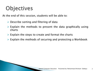
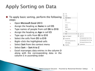
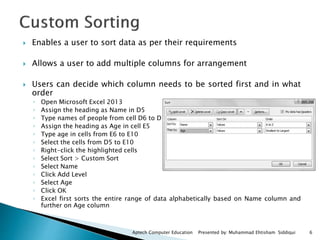
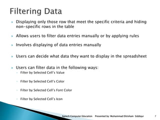
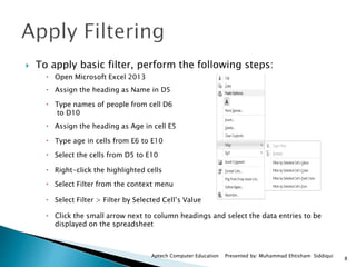

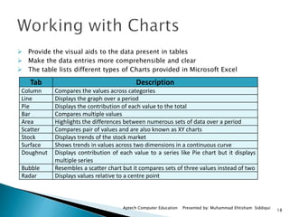
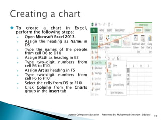


This document discusses data analysis in Microsoft Excel. It covers sorting and filtering data to organize it, presenting data visually using charts, and securing workbooks. Sorting reorganizes rows based on column contents alphabetically or numerically. Filtering displays only certain data entries. Charts like column, line, pie and bar charts can be used to visualize data trends. Formatting options are available to customize charts. Workbooks can be secured when data is confidential.