Download to read offline

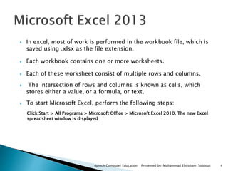
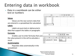
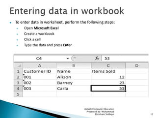
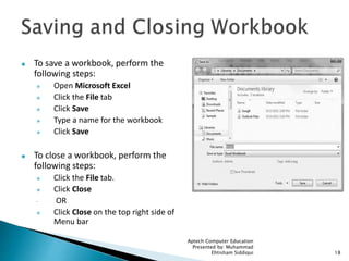
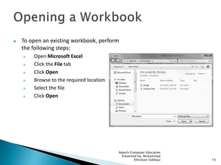
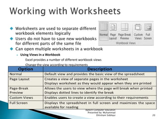
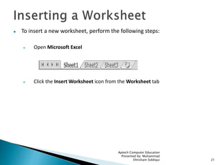
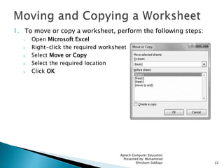
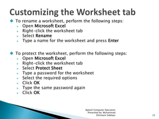


This document provides instructions on how to use Microsoft Excel. It describes the basics of Excel including the elements of the application interface like ribbons, tabs, cells, rows and columns. It explains how to create and open workbooks and worksheets, navigate within a workbook, enter and format data, insert and delete cells and rows, use cut, copy and paste functions, and more. The document is intended to explain the key concepts and procedures for using Excel spreadsheets.