Downloaded 638 times


![Choice of Slave d.o.f All rotational d.o.f Find ratio, neglect those having large values for this ratio If [ M ss ] = 0, diagonal, [K r ] = same as static condensation then there is no loss of accuracy](https://image.slidesharecdn.com/numerical-methods-1211798205859074-8/85/Numerical-Methods-30-320.jpg)


![Eqn. 2 are not true. Eigen values unless P = n If [ ] satisfies (2) and (3),they cannot be said that they are true Eigen vectors. If [ ] satisfies (1),then they are true Eigen vectors. Since we have reduced the space from n to p. It is only necessary that subspace of ‘P’ as a whole converge and not individual vectors.](https://image.slidesharecdn.com/numerical-methods-1211798205859074-8/85/Numerical-Methods-35-320.jpg)


![Aim: Generate (neq x m) modal matrix (Ritz vector). Find k and { u } k for the k th component Let [ ] k = substructure Modal matrix which is nk x n , nk = # of interior d.o.f n = # of normal modes take determined for that structure Assuming ‘l’ structure,](https://image.slidesharecdn.com/numerical-methods-1211798205859074-8/85/Numerical-Methods-39-320.jpg)
![(2) Neq x m [ I ] k,k+1 - with # of rows = # of attachment d.o.f. between k and k+1 = # of columns Ritz analysis: Determine [ K r ] = [R] T [k] [R] [ M r ] = [R] T [M] [R] [k r ] {X} = [M] r +[X] [ ] - Reduced Eigen value problem Eigen vector Matrix, [ ] = [ R ] [ X ]](https://image.slidesharecdn.com/numerical-methods-1211798205859074-8/85/Numerical-Methods-40-320.jpg)


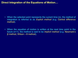
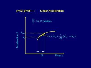
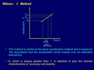
The document summarizes numerical integration methods for solving equations of motion directly in the time domain, including explicit and implicit methods. It describes Newmark's β method, the central difference method, and Wilson-θ method. Key steps involve discretizing the equations of motion and relating response parameters at different time steps using finite difference approximations. Stability, accuracy, and error considerations are also discussed.