The document discusses the fundamentals of 2D plane elasticity using an isoparametric bilinear quadrilateral Lagrange type finite element method. It covers the theoretical background, mathematical formulations, and finite element library related to the method, alongside validation examples and practical applications. The work presented serves as a final presentation by a master's student at the University of Porto's Faculty of Engineering.

![20
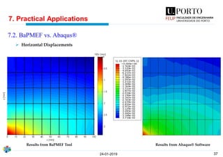
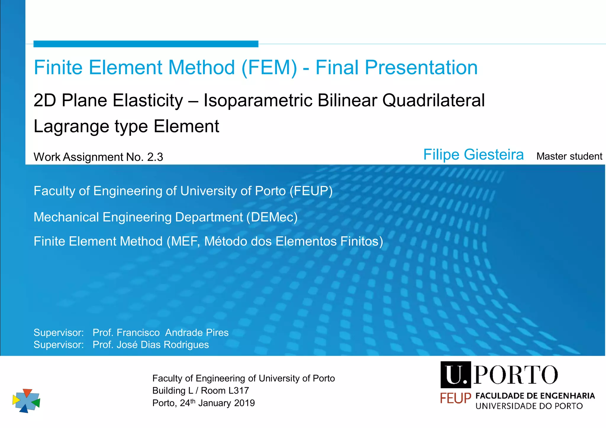
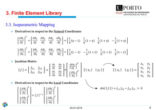
6. Validation Examples
24-01-2019
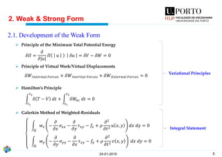
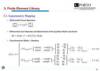
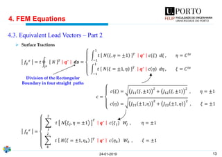
6.1. Constant Rectangular cross-section Beam – Pure Bending
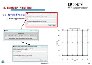
𝑙
𝑙
𝒙 𝒛
𝑢 𝑥, 𝑦 = −
𝑀 𝑜
𝐸𝐼
𝑥𝑦 1 𝑢(𝑥, 𝑦) = −
12𝑀 𝑜
𝐸𝑡𝑤3 𝑥 −
𝑙
2
𝑦 −
𝑤
2
Physical Problem
Equivalent Problem
SimulatedBending Moments ??
Rotation DOF ??
[1] Silva Gomes, Mecânica dos Sólidos e Resistência dos Materiais
Change of Coordinate System
𝑦
𝑥
𝑦
𝑥
𝑤
𝑡
𝑤
𝑀 𝑜 = 𝑃 ∙ 𝑎
Original Coordinate System Coordinate System of the BaPMEF tool](https://image.slidesharecdn.com/isoparametricbilinearquadrilateralelementpptpresentation-190602144941/85/Isoparametric-bilinear-quadrilateral-element-_-ppt-presentation-20-320.jpg)
![21
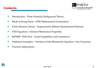
6. Validation Examples
24-01-2019
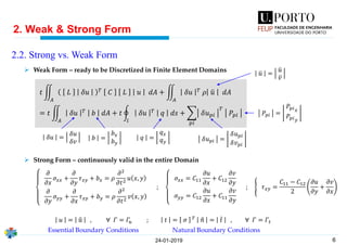
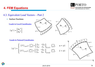
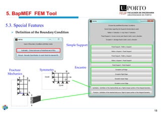
6.1. Constant Rectangular cross-section Beam – Pure Bending
Comparison of
the
displacements in
the x-direction,
determined by
the BaPMEF tool
against the
Analytical
solution
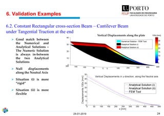
➢ Overall good match
between the Analytical
and Numeric Solution
➢ Null displacements
along the Neutral Axis
➢ Small mismatch near
the plate’s ends:
▪ Analytical
solution badly
behaved in plate’s
boundaries[1]
▪ Boundary
Conditions
difficult to model
in Plane Elasticity
Deformed
shape of
the mesh](https://image.slidesharecdn.com/isoparametricbilinearquadrilateralelementpptpresentation-190602144941/85/Isoparametric-bilinear-quadrilateral-element-_-ppt-presentation-21-320.jpg)
![22
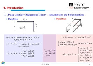
6. Validation Examples
24-01-2019
𝑡
𝑤
𝑢(𝑥, 𝑦) =
𝑃
6𝐺𝐼
𝑦 −
𝑤
2
3
−
𝑃𝑥2
2𝐸𝐼
𝑦 −
𝑤
2
− 𝑣
𝑃
6𝐸𝐼
𝑦 −
𝑤
2
3
+
𝑃𝑙2
2𝐸𝐼
−
𝑃𝑤2
8𝐺𝐼
𝑦 −
𝑤
2
𝑣(𝑥, 𝑦) = 𝑣
𝑃𝑥
2𝐸𝐼
𝑦 −
𝑤
2
2
+
𝑃𝑥3
6𝐸𝐼
−
𝑃𝑙2 𝑥
2𝐸𝐼
+
𝑃𝑙3
3𝐸𝐼
𝑢(𝑥, 𝑦) =
𝑃
6𝐺𝐼
𝑦 −
𝑤
2
3
−
𝑃𝑥2
2𝐸𝐼
𝑦 −
𝑤
2
− 𝑣
𝑃
6𝐸𝐼
𝑦 −
𝑤
2
3
+
𝑃𝑙2
2𝐸𝐼
𝑦 −
𝑤
2
𝑣(𝑥, 𝑦) = 𝑣
𝑃𝑥
2𝐸𝐼
𝑦 −
𝑤
2
2
+
𝑃𝑥3
6𝐸𝐼
−
𝑃𝑙2
2𝐸𝐼
+
𝑃𝑤2
8𝐺𝐼
𝑥 +
𝑃𝑙3
3𝐸𝐼
+
𝑃𝑤2 𝑙
8𝐺𝐼
𝜕𝑣
𝜕𝑥 𝑥=𝑙 ; 𝑦=0
= 0
𝜕𝑢
𝜕𝑦 𝑥=𝑙 ; 𝑦=0
= 0
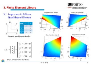
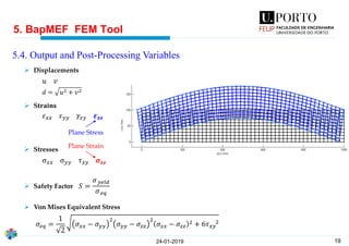
Situation (ii) 1
Situation (i) 1
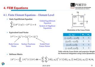
➢ Shear distributed Load
➢ There is no approximation in the definition of the BC
➢ It is also necessary to change the coordinate system
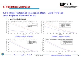
6.2. Constant Rectangular cross-section Beam – Cantilever Beam
under Tangential Traction at the end
[1] Silva Gomes, Mecânica dos Sólidos e Resistência dos Materiais
Problem Simulated
𝑦
𝑥
𝑞
𝑙
𝑤𝑃
𝒒 =
𝑷
𝒘 ∙ 𝒕](https://image.slidesharecdn.com/isoparametricbilinearquadrilateralelementpptpresentation-190602144941/85/Isoparametric-bilinear-quadrilateral-element-_-ppt-presentation-22-320.jpg)
![26
𝑣 𝑥, 𝑦 1
=
𝑸
2𝐸𝐼
൮
൲
𝑦 −
𝑤
2
4
12
−
𝑤2
8
𝑦 −
𝑤
2
2
+
𝑤3
12
𝑦 −
𝑤
2
+ 𝑣
𝑙2
4
− 𝑥 −
𝑙
2
2 𝑦 −
𝑤
2
2
+
𝑦 −
𝑤
2
4
6
−
𝑤2
20
𝑦 −
𝑤
2
2
+
𝑙2
8
𝑥 −
𝑙
2
2
−
𝑥 −
𝑙
2
4
12
−
𝑤2
20
𝑥 −
𝑙
2
2
+
1
4
+
𝑣
8
𝑤2 𝑥 −
𝑙
2
2
−
5𝑙4
192
1 +
12𝑤2
5𝑙2
4
5
+
𝑣
2
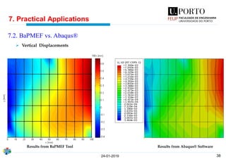
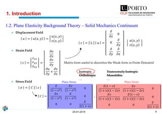
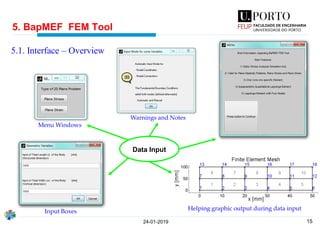
6. Validation Examples
24-01-2019
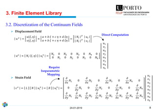
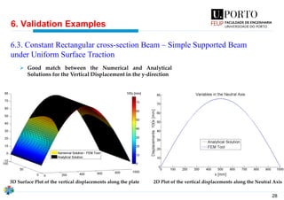
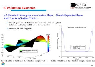
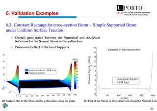
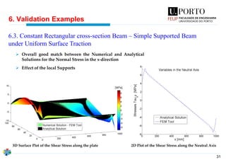
6.3. Constant Rectangular cross-section Beam – Simple Supported Beam
under Uniform Surface Traction
𝑙
𝑤
𝑞
𝑦
𝑥 𝑡
𝑤
𝑞
𝑄
➢ There is no approximation in the definition of the BC
[1] Silva Gomes, Mecânica dos Sólidos e Resistência dos Materiais
Problem Simulated
𝑸 = 𝒒 ∙ 𝒕](https://image.slidesharecdn.com/isoparametricbilinearquadrilateralelementpptpresentation-190602144941/85/Isoparametric-bilinear-quadrilateral-element-_-ppt-presentation-26-320.jpg)
![27
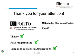
6. Validation Examples
24-01-2019
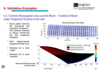
6.3. Constant Rectangular cross-section Beam – Simple Supported Beam
under Uniform Surface Traction
➢ It is also necessary to change the original Coordinate System of the Analytical Solution
➢ Analytical Solutions for the Stresses
𝜎 𝑥𝑥
1 =
𝑸
2𝐼
2
3
𝑦 −
𝑤
2
3
−
𝑤2
10
𝑦 −
𝑤
2
−
𝑸
2𝐼
𝑥 −
𝑙
2
2
−
𝑙2
4
𝑦 −
𝑤
2
𝜎 𝑦𝑦
1 = −
𝑸
2𝐼
𝑦 −
𝑤
2
3
3
−
𝑤2
4
𝑦 −
𝑤
2
−
𝑤3
12
𝜏 𝑥𝑦
1 =
𝑸
2𝐼
𝑦 −
𝑤
2
2
−
𝑤2
4
𝑥 −
𝑙
2
[1] Silva Gomes, Mecânica dos Sólidos e Resistência dos Materiais
Deformed Shape of the Mesh](https://image.slidesharecdn.com/isoparametricbilinearquadrilateralelementpptpresentation-190602144941/85/Isoparametric-bilinear-quadrilateral-element-_-ppt-presentation-27-320.jpg)
![33
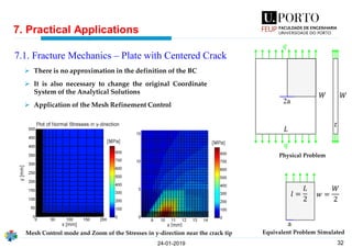
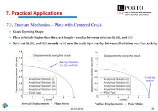
7. Practical Applications
24-01-2019
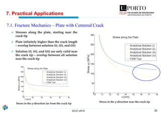
7.1. Fracture Mechanics – Plate with Centered Crack
𝜎 𝑦𝑦 =
𝑞 𝑎
)2(𝑥 − 𝑎
𝜎 𝑦𝑦 =
𝑞 𝑎
)2(𝑥 − 𝑎
sec
𝜋𝑎
𝐿
𝜎 𝑦𝑦 =
𝑞 𝑎
)2(𝑥 − 𝑎
𝐿
𝜋𝑎
tan
𝜋𝑎
𝐿
𝜎 𝑦𝑦 =
𝑞
1 −
𝑎
𝑥
2
4
𝐸
𝑞
𝑎2 − 𝑎𝑥
2
;
4
𝐸
𝑞
𝑎2 − 𝑎𝑥
2
sec
𝜋𝑎
𝐿
;
4
𝐸
𝑞
𝑎2 − 𝑎𝑥
2
𝐿
𝜋𝑎
tan
𝜋𝑎
𝐿
;
2
𝐸
𝑞 𝑎2 − 𝑥2 ;
)4(1 − 𝑣2
𝐸
𝑞
𝑎2 − 𝑎𝑥
2
)4(1 − 𝑣2
𝐸
𝑞
𝑎2 − 𝑎𝑥
2
sec
𝜋𝑎
𝐿
)4(1 − 𝑣2
𝐸
𝑞
𝑎2 − 𝑎𝑥
2
𝐿
𝜋𝑎
tan
𝜋𝑎
𝐿
)2(1 − 𝑣2
𝐸
𝑞 𝑎2 − 𝑥2
Plane Stress Plane Strain Solution [2]
(i)
(ii)
(iii)
(iv)
𝑣 𝑥, 𝑦 =
𝑣 𝑥, 𝑦 =
𝑣 𝑥, 𝑦 =
𝑣 𝑥, 𝑦 =
➢ Plane Strain Problem
[2] David Broke, Elementary Engineering Fracture Mechanics](https://image.slidesharecdn.com/isoparametricbilinearquadrilateralelementpptpresentation-190602144941/85/Isoparametric-bilinear-quadrilateral-element-_-ppt-presentation-33-320.jpg)
![36
7. Practical Applications
24-01-2019
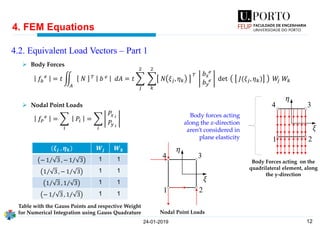
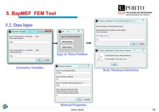
7.2. BaPMEF vs. Abaqus®
15 Τ𝑁 𝑚𝑚2
𝑷
5 Τ𝑁 𝑚𝑚2
150 [𝑁]
500 [𝑁]
50 [𝑁]
100 [𝑚𝑚]
100 [𝑚𝑚]
30 [𝑚𝑚] 30 [𝑚𝑚]
20 [𝑚𝑚] 20 [𝑚𝑚]
10 Τ𝑁 𝑚𝑚2
BaPMEF
➢ Commercially
Available FEA Software
– Abaqus ®
➢ Plane Strain Problem
➢ Generic Loading – No
Analytical Solution
Available
➢ Gravity Body Forces
➢ Surface Tractions acting
along the whole
boundary
➢ Surface Tractions acting
on each Element
Problem
Simulated
in Abaqus
Problem Simulated
in BaPMEF
Gravity Force](https://image.slidesharecdn.com/isoparametricbilinearquadrilateralelementpptpresentation-190602144941/85/Isoparametric-bilinear-quadrilateral-element-_-ppt-presentation-36-320.jpg)