The document is a presentation about navigation and trajectory control for autonomous vehicles. It was presented by two students from the University of Trento in Italy. The presentation introduces mobile robot design considerations including the interrelation between tasks, environments, kinematic models, path/trajectory planning, and high-level and low-level control. It explains that the robot task and environment must be identified first and the kinematic model selected based on this. Path planning is then needed to generate admissible trajectories that satisfy the kinematic constraints. High-level control executes tasks and trajectories while low-level control handles velocity commands. It also explains concepts like holonomic and non-holonomic constraints, accessibility spaces, and maneuvers

1. Navigation and Trajectory Control for
Autonomous Vehicles
Presented by:
Mithun Chowdhury Tesfaye Asmera Mengesha
Matricola No. 160758 Matricola No. 160827
Student of Mechatronics Engineering Student of Mechatronics Engineering
University of Trento, Italy University of Trento, Italy
UNIVERSITY OF TRENTO
2015, Italy

2. Question 1:
Introduce mobile robot designing with considerations about the interrelation existing within:
Task Operational environments Chosen kinematic model Admissible
path/trajectory planning Low-level control High-level control (overall strategy)
Solution:
The design of Mobile robot requires different level of consideration as its mobile base moves
through the environment. Complement to manipulation, the robot arm is fixed but moves objects
in the workspace by imparting force to them. In mobile robotics, the environment is fixed and the
robot moves by imparting force to the environment. Mobile robots have mobile base which
allows it to move freely in the environment.
Tasks and operational environment: Usually the mobile robot task and operational
environment is two completely related terms that goes together. Identification of required task to
be executed is the first step in design of mobile robot. The tasks can be a combination of high
level tasks and low level tasks depending on the application area. The tasks are accomplished
carrying out high level procedures executed concatenating with simpler low level execution. The
execution of mobile robot task is in operational environment, which could be structured
environment or unstructured environment in which there exists no obstacles or static obstacles or
moving objects. Depending on the tasks to be completed and the operational environments a
robot suitable for that application area is designed. This helps for selection of kinematic model of
the robot. So, after identifying the robot and the tasks, task planning should be developed. With
the robot moving in the operational environment the path which fulfills the needed criteria has to
be planned. Path planning is one of the key steps in mobile robot design for execution of the task
in a given operational environment. Trajectory is admissible trajectory if it can be a solution of
kinematic model. Admissible trajectory is the extension of admissible path with introduction of
time law. Planning produces a set of inputs for control loops. The control loop employs high
level control to execute high level tasks and meet the requirement of the robot. It is purely
kinematics based. In the mean while low level control is adopted for low level tasks.
Kinematic model choice: kinematics is the basic study of how the mechanical system of robot
behaves. In mobile robotics, we need to understand the mechanical behavior of the robot both in
order to design appropriate mobile robots for tasks and to understand how to create control
software for an instance of mobile robot hardware.
The kinematic model of a wheeled mobile robot must satisfy the non-holonomic constraints
imposed due to rolling without slipping condition. Denoting input vector fields by {g1,...,gm.} a
basis of N(AT
(q)), the admissible trajectories for the mechanical system can then be
characterized as the solutions of the non-linear dynamical system.

3. ( ) ( )
1
m
gj q uj G q uq
j




, m = n – k
Where q Rn
is the state vector and u = [u1…um]T
IRm
is the input vector. The choice of the
input vector fields g1 (q),...,gm(q) is not unique. Correspondingly, the components of u may
have different meanings. In general, it is possible to choose the basis of N (AT
(q)) in such a way
that the uj have a physical interpretation. In any case, vector u may not be directly related to
the actual control inputs that are generally forces and torques.
The holonomy or nonholonomy of constraints can be established by analyzing the controllability
properties of the associated kinematic model.
Admissible path/trajectory planning: admissible path is the path which fits to the desired
kinematic model whereas admissible trajectory is the extension of the path with associated time.
The path/trajectory is said to be Admissible path or trajectory if it is the solution of kinematic
model. With the robot moving in the operational environment the path which fulfills the needed
criteria has to be planned. Now, we can define Admissible Path as a solution of the differential
system corresponding to the kinematic model of the mobile robot, with some initial and final
given conditions. In other words, robot must meet the boundary condition (interpolation of the
assigned points and continuity of the desired degree) and also satisfy the non-holonomic
constraints at all points.
Planning: for execution of specific robotic task involves the consideration of motion planning
algorithm. In wheeled mobile robot path and trajectory (path with associated time law) planning
involves the admission flat output y and its derivative to certain order. The goal of non-
holonomic motion planning is to provide collision-free admissible paths in the configuration
space of the mobile robot system. Many kinematic models of mobile robots, including the
unicycle and the bicycle, exhibits a property known as differential flatness, that is particularly
relevant in planning problems. A non-linear dynamic system
( ) ( )*X f x G x u

 
is said to be differentially flat if there exists a set of output y, called flat outputs, such that the
state x and the control inputs u can be expressed algebraically as a function of y and its time
derivatives up to certain order:
( )
( , , ,.... )
r
x x y y y y
 

( )
( , , ,.... )
r
u u y y y y
 


4. Based on the assignment of output trajectory to flat output y, the associated trajectory of the state x and
history of control inputs u are uniquely determined. In fact Cartesian coordinates of unicycle and bicycle
mobile robot is flat output.
Path planning problem can be solved efficiently whenever the mobile robot admits the set of flat output.
The path can be planned by using interpolation scheme considering the satisfaction of boundary
condition. Approaches of path planning:
Planning via Cartesian polynomials
Planning via the chained form
Planning via the parameterized inputs
For example in the following considered vehicle is a unicycle that must perform various parking
manoeuvores.
Figure 1. These results shows two parking manoeuvres planned via cubic Cartesian polynomials; with the
same forward motion.
After the path q, q [qi, qf] has been determined the it is possible to choose a timing law q = q(t) with
which the robot should follow it. For example in the case of unicycle if the driving velocity and steering
velocity is subjected to the bounds,
max( )v t v
max( )t 
It is necessary if the velocities along the planned path are admissible. The timing law is rewritten by
normalizing the time variable  as follows, /t T  with T = tf- ti
1
( ) ( )
ds
v t v s
dt T
 ,
1
( ) ( )
ds
t s
dt T
 
Increasing the duration of trajectory, T, reduces the uniformity of v and .

5. High level control: High level control purely kinematics-based, with velocity commands for wheeled
mobile robots (WMR). In WMR it is dedicated to generate reference motion (VL and VR), display user
interface with real-time visualization as well as a simulation environment. The objective of high level
control in mobile robots can be summarized as:
Use sensor data to create model of the world
Use model to form a sequence of behaviors which will achieve the desired goal
Execute the plan
Low-level control loops: These loops that are integrated in the hardware or software architecture, accepts
as input a reference value for the wheel angular speed that is reproduced as accurately as possible by
standard regulation actions (e.g., PID controllers). The low-level control layer is in charge of the
execution of the high-level velocity commands.
PID controller for motor velocity
PID controller for robot drive system
Overall strategy: The overall strategy is to implement the control of the mobile robot based on a two
level hierarchy in which the high level is dedicated to generating the inputs that are required to execute a
planned path. WL and WR are the wheel angular velocity required at that instant of time, while the low
level control is dedicated to executing the velocity commands coming from high level control. One good
example available in literatures is the wheeled mobile robot superMario. SuperMARIO is a two-wheel
differentially-driven vehicle, which more kinematically stable but equivalent form of a unicycle model.
The high level control is dedicated in path planning and generating reference velocities while the low
level control, can be the PID controls the wheel motor.
Figure 2. Overall strategy of mobile robot design

6. Question 2:
Explain the interrelations within:
Position and/or velocity constraints; (non)holonomicity; (non)integrability; (non)involutivity; in-
stantaneous motion directions; local/global accessibility and manoeuving.
Solution:
In mobile robotics, we need to understand the mechanical behavior of the robot both in order to
design appropriate mobile robots for tasks and to understand how to create control software for an
instance of mobile robot hardware. It is subject to kinematic constraints that reduce in general its
local mobility, while leaving intact the possibility of reaching arbitrary configurations by appro-
priate maneuvers. The motion of the system that is represented by the evolution of configuration
space over time may be subject to constraints. Position constraint reduces the positions that can be
reached by the robot in the configuration space, i.e. they are related to the generalized coordinates.
Thus, these constraints reduce the configuration space of the system. Velocity constraints reduce a
set of generalized velocities that can be attained at each configuration.
In the robotics community, when describing the path space of a mobile robot, often the concept
of holonomy is used. The term holonomic has broad applicability to several mathematical areas,
including differential equations, functions and constraint expressions. In mobile robotics, the term
refers specifically to the kinematic constraints of the robot chassis. A holonomic robot is a robot
that has zero non-holonomic kinematic constraints. Conversely, a non-holonomic robot is a robot
with one or more non-holonomic kinematic constraints.
Let, q = [q1 ...q2 ...qn], i = 1,...,k < N with qgeneralized coordinates and εRN and hi : C → R
are of class C∞
order (smooth) and independent.
A kinematic constraint is a holonomic constraint if it can be expressed in the form∑hi = H(q) = 0
i
Kinematic constraints formulated via differential relations (constant in velocity) are holonomic if
they are integrable A(q, ˙q) = 0. In the of holonomic systems, we obtain N differential Pfaffian
constraints. Holonomic constraints reduce the space of accessible configuration from n to n-k be-
cause the motion of the mechanical system in configuration space is confined to a particular level
surface of the scalar functions Thus, they can be characterized as position constraints. Holonomic
constraints are generally the result of mechanical interconnections between the various bodies of
the system. A mobile robot with no constraints is holonomic. I A mobile robot capable of only
translations is also holonomic.
Constraints that involve generalized coordinates and velocities are called kinematic constraints.
Kinematic constraints are generally linear in generalized velocities. If kinematic constraint is
not integrable, it is called non-holonomic. Thus, non-integrablity of kinematic constraint implies

7. non-holonomic nature of that constraint. Non-holonomic constraints reduce the mobility of the
mechanical system in a completely different way with respect to holonomic constraints. These
constraints involve generalized coordinates and velocities and constrain the instantaneous admis-
sible motion of the mechanical system by reducing the set of generalized velocities that can be
attained at each configuration. Non-holonomic constraints are non integrable. One of the test that
gives us information the system nonholomicity is the involutibvity test obtained via Lie algebra
and Froboenius involutivity theorem.
Definition 1: For two vector fields f and g, the Lie bracket is a third vector field defined by:
[f,g](q) =
∂g
∂q
f(q)−
∂ f
∂q
g(q)
It is obvious that [f, g] = −[f, g] = 0 for constant vector fields f and g.
Definition 2: A distribution ∆is involutive if it is closed under Lie bracket operation, that is,
if
g1ε∆ and g2ε∆ ⇒ [g1,g2]ε∆
For a distribution ∆ = span{g1 ..., g2}, where gi is the basis of N(AT (q)), the distribution is invo-
lutive if it is closed under Lie brackets.
Frobenius’s theorem: A regular distribution is integrable if and only if it is involutive.
The mobile robot maneuverability is the overall degrees of freedom that a robot can manipulate. It
can also be defined in terms of mobility and steerability. Maneuverability includes both the degrees
of freedom that the robot manipulates directly through wheel velocity and the degrees of freedom
that it indirectly manipulates by changing the steering configuration and moving.
7

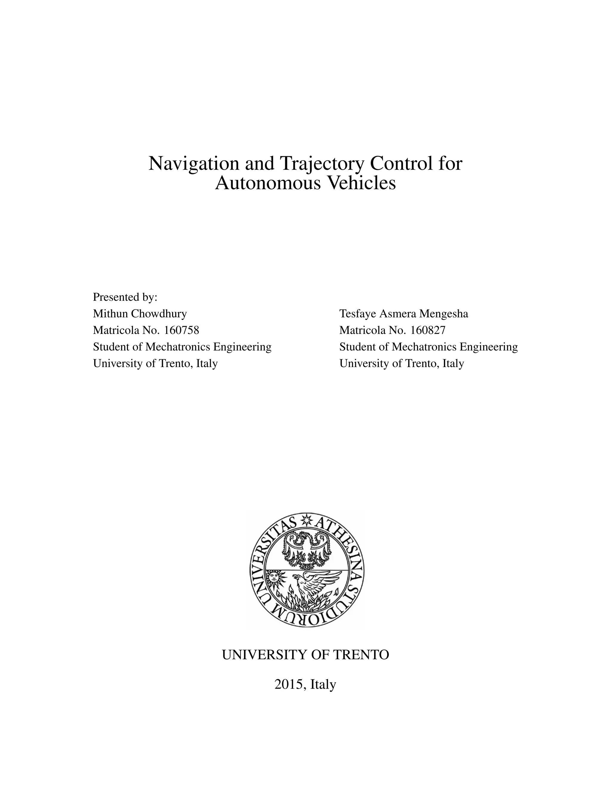
8. Question 3:
Compute the accessibility space for the following representative kinematic models after having
re-obtained them from the original kinematic equations
• Unicycle (ideal -single wheel) (U)
• Car-like front-driven (FD); or alternatively:
• Car-like rear-driven (RD)
• Rhombic-like vehicles (RLV)
Solution:
A. Unicycle (ideal - single wheel) (U):
A unicycle is a vehicle with a single orientable wheel.
Figure 1:
Its configuration can be described by three generalized coordinates: the Cartesian coordinates (x,y)
of the contact point with the ground, measured in a fixed reference frame; angle θ characterizing
the orientation of the disk with respect to the x axis.
The configuration vector is thereforeq = [xyθ]T . The kinematic constraint of unicycle is derived
from the rolling without slipping condition, which forces the unicycle not to move in the direction
orthogonal to the sagittal axis of the vehicle. The angular velocity of the disk around the vertical
axis instead is unconstrained.
.
x sinθ−
.
y cosθ = 0
=⇒ sinθ −cosθ 0
.
q= 0
This equation is nonholonomic, because it implies no loss of accessibility in the configuration
space. Now, here the number of generalized coordinate, n = 3 and the number of non-holonomic
8

9. constraints, k = 1. So the number of null space of kinematic constraints in the case of unicycle,
m = n−k = 2. Thus the matrix:
G(q) = [g1(q) g2(q)] =



cosθ 0
sinθ 0
0 1


,
where, columns g1(q) and g2(q) are for eachq a basis of the null space of the matrix associated
with the Pfaffian constraint.
The kinematic model of the unicycle is then
.
q=



.
x
.
y
.
θ


 =



cosθ
sinθ
0


v+



0
0
1


ω,
where the input v is the driving velocity and ω is the wheel angular speed around the vertical axis.
The Lie bracket of the two input vector field is
[g1,g2](q) =



sinθ
−cosθ
0


,
that is linearly independent from g1(q), g2(q). The Accessibility space, S = rank g1 g2 [g1,g2] =
3. This indicates that there is no loss in the accessible space and the constraint is non-holonomic.
9

10. Figure 2:
B. Car-like front-driven (FD):
A bicycle vehicle consists of an oreintable wheel and a fixed wheel.
The generalized coordinates can be expressed by the following equation:
q = x y θ Φ
T
, where (x,y) are the cartesian coordinates of the contact point between
the rear wheel and the ground, and θ is the steering angle of the front wheel with respect of the
vehicle. The kinematic model is derived from the two pure rolling constraints. The velocity of the
centre of the front wheel is zero in the direction orthogonal to the wheel itself, while the velocity
of the centre of the rear wheel is zero in the direction orthogonal to the sagittal axis of the vehicle.
Now using the rigid body constraint,
xf = x+lcosθ
yf = y+lsinθ
where, l is the distance between the wheels and (xf ,yf ) is the cartesian position of the centre of
the front wheel. So two constraints are following:
.
x sinθ−
.
y cosθ = 0 and
.
xf sin(θ +Φ)−
.
yf cos(θ +Φ) = 0
⇒
.
x sin(θ +Φ)−
.
y cos(θ +Φ)−l
.
θ cosΦ = 0
The matrix associated with the Pfaffian constraints is then:
AT
(q) =
sinθ −cosθ 0 0
sin(θ +Φ) −cos(θ +Φ) −lcosΦ 0
withrank2
10

11. Here the number of generalized coordinate, n = 4 and the number of non-holonomic constraints,
k = 2. So the number of null space of kinematic constraints in the case of unicycle, m = n−k = 2.
Thus the matrix,
G(q) = [g1(q) g2(q)] =





cosθcosΦ 0
sinθsinΦ 0
sin(Φ/l) 0
0 1





where, columns g1(q) and g2(q) are for eachq a basis of the null space of the matrix associated
with the Pfaffian constraint. The kinematic model of the unicycle is then,
.
q=





.
x
.
y
.
θ
.
Φ





=





cosθcosΦ
sinθsinΦ
sin(Φ/l)
0





v+





0
0
0
1





ω
where, the input v is the driving velocity of front wheel and ω is the steering velocity. Now the Lie
bracket,
g3(q) = [g1,g2](q) =





cosθcosΦ
sinθsinΦ
−cos(Φ/l)
0





g(q) = [g1,g3](q) =





−sin(θ/l)
cos(θ/l)
0
0





both linearly independent from g1(q) and g2(q). So, the Accessibility space, S = rank g1 g2 g3 g4 =
4.
11

12. C. car like rear-driven (RD)
The robot is rear driven for a possible generalized coordinates of [ ] T where (x, y) are
the Cartesian coordinates of the contact point between the rear wheel and the ground (i.e., of the
rear wheel Centre), θ is the orientation of the vehicle with respect to the x axis, and φ is the
steering angle of the front wheel with respect to the vehicle.
Front wheel center is
and
̇ ̇ ̇
̇ ̇ ̇
Applying rolling without slipping condition on the front axle/wheels,
̇ ( ) ̇ ( )
Substituting the above equations,
( ̇ ̇ ) ( ) ( ̇ ̇ ) ( )
Solving for ̇ gives, ̇
The complete kinematic model is given by,

13. [
̇
̇
̇
̇
]
[ ]
v + [ ]
This is the complete kinematic model of Car like rear driven (RD) mobile robot where v is the
driving velocity of rear wheel whereas is the steering velocity.
Accessible space = Rank [g1, g2, [g1, g2], [g1, [g1, g2]]]
g1(q) =
[ ]
and g2(q) = [ ]
g3 (q) = [g1, g2] (q) =
[ ]
g4 (q) = [g1, g3] (q) =
[ ]
So from the computed result g3(q) and g4(q) vector fields are independent of g1(q) and g2(q).
This implies that the accessible space = Rank[g1,g2,g3,g4] = 4
D. rhombic like vehicles (RLV)
In the configuration of RLV using the assumption of rolling without slipping condition the
system is subjected to the following constraints:
̇ ( ) ̇ ( )
̇ ( ) ̇ ( )
Using rigid body constraints, ̇ ̇ can be obtained as the function of center mass ̇ .thus

14. [ ], C (q) ̇ = 0
[
( ) ( )
( ) ( )
] [
̇
̇ ]= 0
̇ is the basis of {N(C (q))} = ∑ ( )
Null space of C(q) :g1(q) =
[
( )
( )
]
, g2(q)=
[
( )
( )
]
̇
[
( )
( )
]
+
[
( )
( )
]
This is the kinematic model of RLV
Accessible space = rank [g1, g2,[g1,g2]]
[ ] = [
( ( ) ( ) )
( ) ]
Since [g1,g2] is independent of g1 and g2, accessible space = 3.
Advantages of pfaffian constraint:
Pfaffian constraints are linear in generalized velocities:
( ) ̇
This gives us the advantages of expressing the kinematic model as the combination of null space
of the constraint: in this case the kinematic model is drifless system.

15. Question 4:
MATLAB exercise - path/trajectory planning and potentials
Motion planning: It is the process of breaking down a desired movement task into discrete motions
that satisfy movement constraints and possibly optimize some aspect of the movement as well as
avoid obstacles. In the original package given to us in order to move the robot from a given initial
point to goal point, a motion planning algorithm is developed for random environment map and
minimum time path is computed using constrained optimization. The motion planning algorithm
generates path/trajectory based on polynomial interpolation of waypoints from starting position to
goal position. The minimum time path is computed by constrained optimization of the path gener-
ated based on the waypoints randomly chosen. This optimization algorithm provides the optimal
waypoints between starting position and goal. But, the package doesn’t consider about the pres-
ence of obstacles when making the environment and so, the final path/trajectory is always straight
line connecting the two points.
Modification:
• the mapping environment is structured
• known position of obstacles are randomly imposed.
0 5 10 15 20 25 30 35
−5
0
5
10
15
20
25
−1
−0.8
−0.6
−0.4
−0.2
0
0.2
0.4
0.6
0.8
1
Figure: Environment map with obstacles, indicating the starting point and end point
15

16. 0 5 10 15 20 25 30 35
−5
0
5
10
15
20
25
0
0.05
0.1
0.15
0.2
0.25
0.3
0.35
0.4
0.45
Figure: Search note
0 5 10 15 20 25 30
0
5
10
15
−1
−0.8
−0.6
−0.4
−0.2
0
0.2
0.4
0.6
0.8
1
Figure: Optimal points on the map
0 5 10 15 20 25 30 35
−5
0
5
10
15
20
25
0
0.05
0.1
0.15
0.2
0.25
0.3
0.35
0.4
0.45
Figure: Optimal path
16

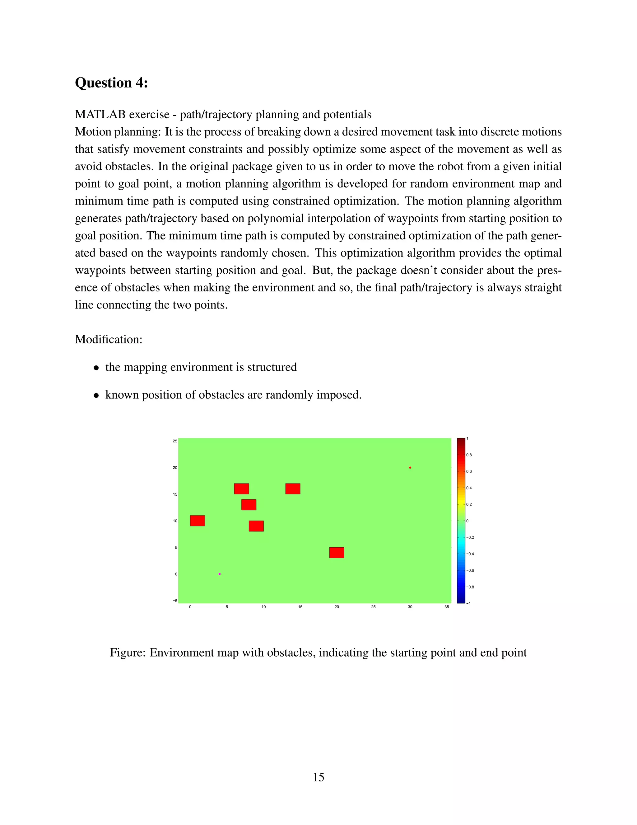
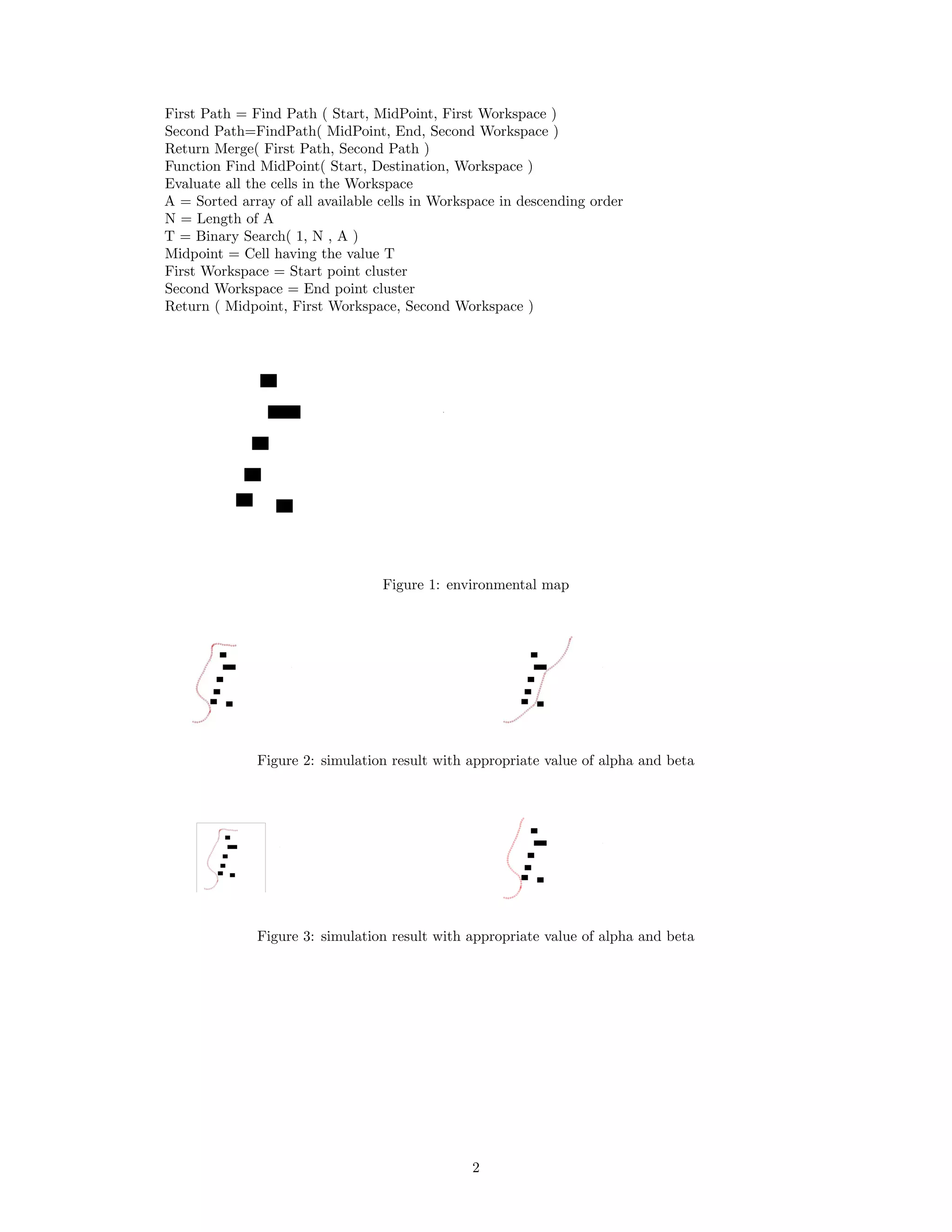
17. Question 04 (Extension of Path Planning)
Iterative artificial potential field (APF) algorithm APF algorithm is built upon new potential
functions based on the distances from obstacles, destination point and start point. The algorithm
uses the potential field values iteratively to find the optimum points in the workspace in order to
form the path from start to destination. The number of iterations depends on the size and shape of
the workspace.
In this algorithm the map is assumed to be captured by camera mounted on the robot. For the
sake of simulation environmental map is generated by using customized function and changed into
environmental map. The obstacles repel the robot with the magnitude inversely proportional to
the distances. The goal attracts the robot. The resultant potential, accounting for the attractive
and repulsive components is measured and used to move the robot. five distances are measured at
specific angles to to compute the repulsive potential. These are are forward ,left side right side, left
diagonal and forward right diagonal.
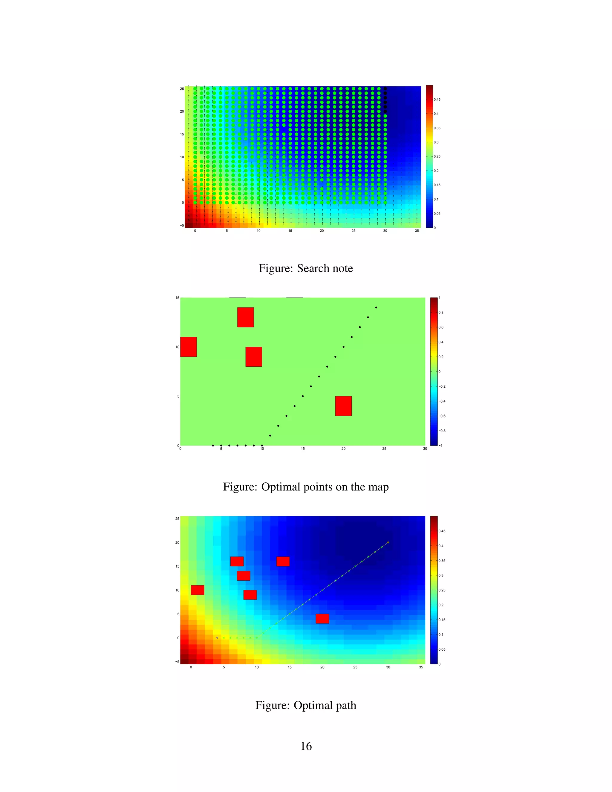
Our method involves using a simple potential functions; the workspace is discretized into a grid of
rectangular cells where each cell is marked as an obstacle or a non-obstacle. At each cell potential
function is evaluated based on the distances from the starting point, destination and goal. These
values are used to find the optimum points along the entire path. We find these points iteratively
until there are enough points that path can be determined as a consecutive sequence of these points
beginning from the start location and ending at the destination.
each cell by its coordinates c = [x, y]. Algorithm begins calculating the potential function for every
empty cell in the workspace. UT otal(c) = UStart(c) + UEnd(c)UObs(c) It is important to note that
the distance of the cell from the start point is being used. The individual functions are expressed as
UStart(c) = α/D(c, start)
UEnd(c) = α/D(c, End)
UObs(c) = β/D(c, Obs)
D(c, start) is the distance of the cell c from the start point D(c, End) is the distance of cell c from
the end point D(c, Obs) is the distance of cell c from the Obstacle point
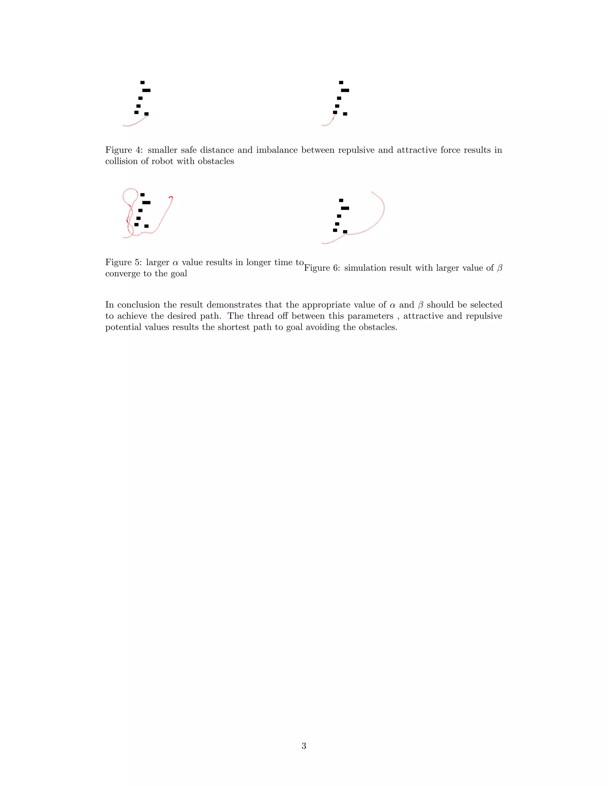
α and β are positive constant to change the path behavior. As it can be observed from potential
function by increasing alpha we put more emphasis on the distance from the start and end points.
So having large value of alpha results in shorter path but the path might be close to the obstacle.
By increasing beta we put more emphasis on the distance from obstacles and it means that selecting
large value for gives us a longer path with bigger distance from the obstacles. For this simulation
result in the documentation unit value of alpha and beta. Pseudo code for finding the midpoint Let
N be the number of available cells, Evaluate all these cells. A = Sorted array of all cells values.
Binary Search( 1, N , A );
Binary Search( i, j ,A)
If ( i == j )
return A[ i + 1]
T = A[ ( i + j ) / 2]
If ( by using simple BFS, Is end point reachable from start point using cells with larger value than
T ? )
Binary Search( i, (( i + j ) / 2 ) - 1 , A )
Else
Binary Search( ( i + j ) / 2, j, A )
Pseudo code for finding the path
Inputs = Start, Destination, Workspace
Output = Collision free path
Function Find Path (Start, End, Workspace)
If ¡ Endpoints are close enough and there is a collision free straight line connecting them ¿
Return Segment( Start, End );
Else
[ MidPoint, First Workspace, Second Workspace] = Find MidPoint( Start, End, Workspace )
1

18. First Path = Find Path ( Start, MidPoint, First Workspace )
Second Path=FindPath( MidPoint, End, Second Workspace )
Return Merge( First Path, Second Path )
Function Find MidPoint( Start, Destination, Workspace )
Evaluate all the cells in the Workspace
A = Sorted array of all available cells in Workspace in descending order
N = Length of A
T = Binary Search( 1, N , A )
Midpoint = Cell having the value T
First Workspace = Start point cluster
Second Workspace = End point cluster
Return ( Midpoint, First Workspace, Second Workspace )
Figure 1: environmental map
Figure 2: simulation result with appropriate value of alpha and beta
Figure 3: simulation result with appropriate value of alpha and beta
2

19. Figure 4: smaller safe distance and imbalance between repulsive and attractive force results in
collision of robot with obstacles
Figure 5: larger α value results in longer time to
converge to the goal
Figure 6: simulation result with larger value of β
In conclusion the result demonstrates that the appropriate value of α and β should be selected
to achieve the desired path. The thread off between this parameters , attractive and repulsive
potential values results the shortest path to goal avoiding the obstacles.
3

20. Question 5:
5.1 Produce a “sufficiently smooth” path planning and trajectory?
Trajectory planning involves path planning with association of timing law.
Assuming the trajectory to be planned q (t), for t ∈ [ti , tf], that leads a car like robot from an initial
Configuration q(ti ) = qi to a final configuration q(tf) = qf in the absence of obstacles. The trajectory
q(t) can be broken down into a geometric path q(s), with dq(s)/ds = 0 for any value of s, and a
timing law s=s(t), with the parameters varying between s(ti)=si and s(tf)=sf in a monotonic fashion,
i.e., with s(t) ≥0, for t ∈[ti, tf]. A possible choice for s is the arc length along the path; in this
case, it would be si = 0 and sf =L, where L is the length of the path.
Using space time separation:
𝑞̇ =
𝑑𝑞
𝑑𝑡
=
𝑑𝑞
𝑑𝑠
𝑠̇ = 𝑞′𝑠̇
And the non-holonomic constraints of the rear driven car like robot is given by
𝐴(𝑞) ∗ 𝑞̇ = 𝑞′𝑠̇
Geometrically admissible paths can be explicitly defined as the solutions of the nonlinear system
𝑞′
𝑠̇ = 𝐺(𝑞) ∗ 𝑢̃ , 𝑢 = 𝑠̇ (𝑡)𝑢̃
In this project the path planning via Cartesian polynomial is adopted. The problem of planning can
be solved by interpolating the initial values xi and yi and the final values xf and yf of the flat
outputs x, y. The expression for other states and input trajectory depend only on the values of
output trajectory and its derivative up to third order. In order to guarantee it’s exact
Reproducibility, the Cartesian trajectory should be three times differentiable almost everywhere.
Cubic polynomial function is given as shown below,
𝑥(𝑠) = 𝑠3
∗ 𝑥𝑓 − (𝑠 − 1)3
∗ 𝑥𝑖 + 𝛼 𝑥 ∗ 𝑠2
∗ (𝑠 − 1) + 𝛽 𝑥 ∗ 𝑠 ∗ (𝑠 − 1)2
𝑦(𝑠) = 𝑠3
∗ 𝑦𝑓 − (𝑠 − 1)3
∗ 𝑦𝑖 + 𝛼 𝑦 ∗ 𝑠2
∗ (𝑠 − 1) + 𝛽 𝑦 ∗ 𝑠 ∗ (𝑠 − 1)2
The constraint equation on the initial and velocities comes from the kinematic model of the robot.
Considering the forward velocity the configuration parameters of the robot becomes as shown in
the following description.
𝜃(𝑠) = atan(𝑥′(𝑠), 𝑦′(𝑠)) 𝑣(𝑠) = √𝑥(𝑠)2 + 𝑦(𝑠)2
∅ = 𝑡𝑎𝑛−1
(𝑙 ∗ 𝑣 ∗ 𝜃(𝑠)̇ )
∅ = arctan (
𝑦(𝑠)̈ 𝑥(𝑠)̇ –𝑥(𝑠)̈ 𝑦(𝑠)̇
√𝑥(𝑠)2+𝑦(𝑠)2
3 )
Adding the timing law to by computing the length of Euclidean distance (L ) between initial and
final position given the speed value V becomes as shown,
L =|‖(𝑥𝑓, 𝑦𝑓) − ((𝑥𝑖, 𝑦𝑖))‖| , Tf =
𝑉
𝐿
and timing Law 𝑠(𝑡) =
𝑉∗𝑡
𝐿

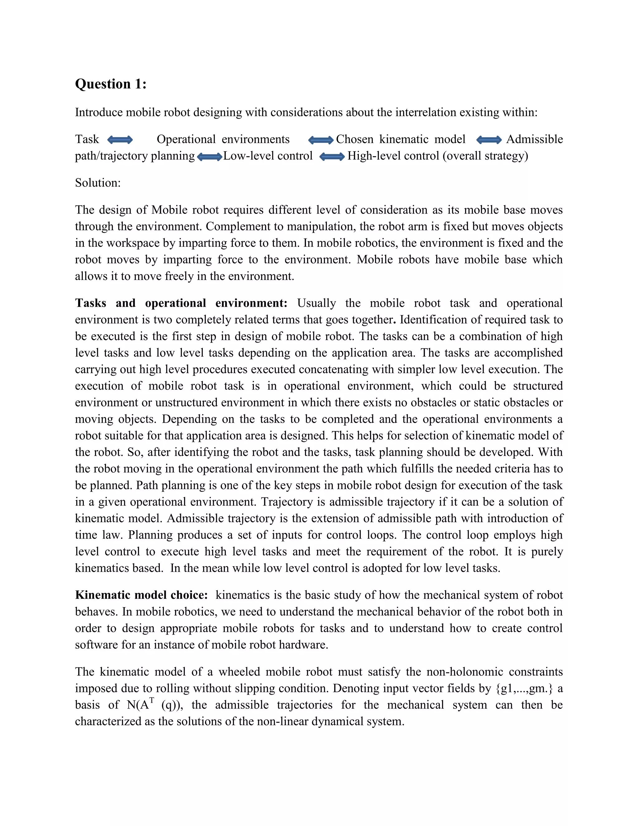
21. 1 1.5 2 2.5 3 3.5 4 4.5
1
1.5
2
2.5
3
3.5
4
Sufficiently smooth path planning
xd
yd
Figure: Maneuvering; Initial configuration, qi = [1 1 pi*0.5 0]; Final configuration, qf = [4 4 -pi
0];
0 0.1 0.2 0.3 0.4 0.5 0.6 0.7
−40
−30
−20
−10
0
10
20
30
40
Steering velocity
s
Wd
Figure: Steering Velocity; Initial configuration, qi = [1 1 pi*0.5 0]; Final configuration, qf = [4 4
-pi 0];
21

22. 0 0.1 0.2 0.3 0.4 0.5 0.6 0.7
0
2
4
6
8
10
12
14
Forward velocity
s
vd
Figure: Forward Velocity; Initial configuration, qi = [1 1 pi*0.5 0]; Final configuration, qf = [4 4
-pi 0];
0.5 1 1.5 2 2.5 3 3.5 4 4.5
1
1.5
2
2.5
3
3.5
4
Sufficiently smooth path planning
xd
yd
Figure: Parralel maneuvering; Initial configuration, qi = [1 1 0 0]; Final configuration, qf = [4 4 0
0]
22

23. 0 0.1 0.2 0.3 0.4 0.5 0.6 0.7
−1
−0.5
0
0.5
1
1.5
2
2.5
3
3.5
4
Steering velocity
s
Wd
Figure: Steering Velocity; Initial configuration, qi = [1 1 0 0]; Final configuration, qf = [4 4 0 0]
0 0.1 0.2 0.3 0.4 0.5 0.6 0.7
6
7
8
9
10
11
12
Forward velocity
s
vd
Figure: Forward Velocity; Initial configuration, qi = [1 1 0 0]; Final configuration, qf = [4 4 0 0]
23

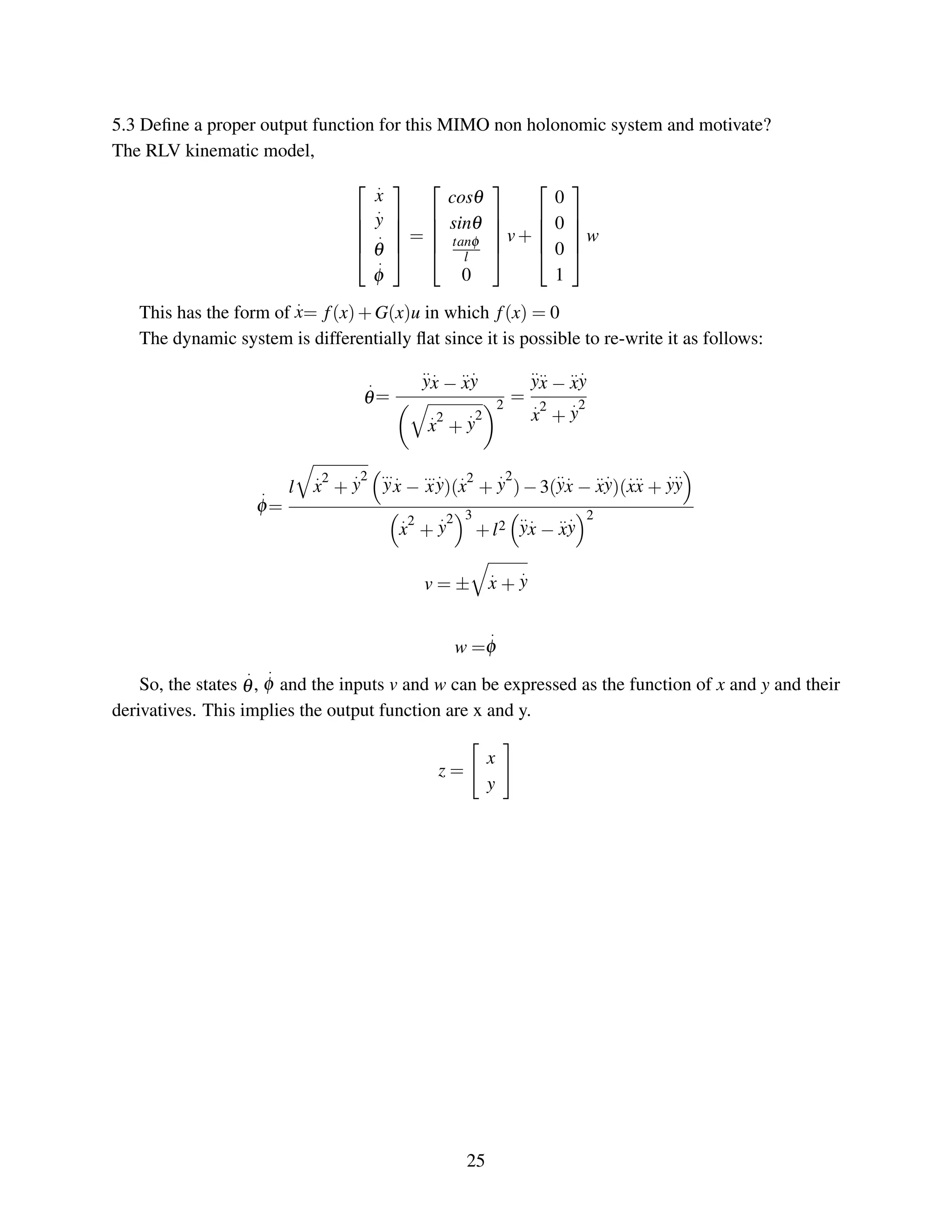
24. 5.2. Compute the kinematic model inputs in order to allow the FR model to follow the assigned
path in the assigned time interval, parameterize the time law, possibly at any step.
From timing law the trajectory i.e the path with associated time law is given by
S(t)=
𝑘𝑡
𝐿
Where k is the initial velocity and L is the length of the path.
In this case the time step is
𝑑𝑡 =
𝑡𝑓 − 𝑡𝑖
1000
The model inputs are the driving velocity and the steering velocity which are the solution of
[
𝑥̇ = 𝑣̃𝑠𝑖𝑛𝜗
𝑦̇ = 𝑣̃𝑠𝑖𝑛𝜗
𝜗̇ =
𝑣̃𝑡𝑎𝑛∅
𝑙
∅̇ = 𝜔̃ ]
𝑣̃ and 𝜔̃ are geometric inputs.
So 𝑣̃(𝑠) = √𝑥′(𝑠)2 + 𝑦′(𝑠)2
𝜔̃( 𝑠)
=
𝑙 𝑣̃(𝑠)[(𝑦′′′(𝑠)𝑥′(𝑠) − 𝑥′′′(𝑠)𝑦′(𝑠)) − 3(𝑦′′(𝑠)𝑥′(𝑠) − 𝑥′′(𝑠)𝑦′(𝑠) )(𝑥′′(𝑠)𝑥′(𝑠) − 𝑦′′(𝑠)𝑦′(𝑠)]
𝑣̃(𝑠)6 + 𝑙2 (𝑦′′(𝑠)𝑥′(𝑠) − 𝑥′′(𝑠)𝑦′(𝑠))
𝑣(𝑡) = 𝑣̃(𝑠)𝑠′(𝑡) = 𝑣̃(𝑠)
𝑘
𝑙
𝜔(𝑡) = 𝜔̃(𝑠)𝑠′(𝑡) = 𝜔̃(𝑠)
𝑘
𝑙

25. 5.3 Define a proper output function for this MIMO non holonomic system and motivate?
The RLV kinematic model,





.
x
.
y
.
θ
.
φ





=





cosθ
sinθ
tanφ
l
0





v+





0
0
0
1





w
This has the form of
.
x= f(x)+G(x)u in which f(x) = 0
The dynamic system is differentially flat since it is possible to re-write it as follows:
.
θ=
..
y
.
x −
..
x
.
y
.
x
2
+
.
y
2
2
=
..
y
..
x −
..
x
.
y
.
x
2
+
.
y
2
.
φ=
l
.
x
2
+
.
y
2 ...
y
.
x −
...
x
.
y)(
.
x
2
+
.
y
2
)−3(
..
y
.
x −
..
x
.
y)(
.
x
..
x +
.
y
..
y
.
x
2
+
.
y
2 3
+l2
..
y
.
x −
..
x
.
y
2
v = ±
.
x +
.
y
w =
.
φ
So, the states
.
θ,
.
φ and the inputs v and w can be expressed as the function of x and y and their
derivatives. This implies the output function are x and y.
z =
x
y
25

26. 5.4. Apply the input output linearization feedback by computing the linearizing feedback via lie
algebra from new coordinates z. rewrite the equation in the old set of generalized coordinates q.
For the car-like robot model, the natural output choice for the trajectory tracking task is
𝑧 = [
𝑥
𝑦]
The linearization algorithm starts by computing
𝑧 = [
𝑐𝑜𝑠𝜃 0
𝑠𝑖𝑛𝜃 0
] 𝑣 = 𝐴(𝜃)𝑣
At least one input appears in both components of 𝑧̇, so that A(𝜃) is the actual decoupling matrix
of the system. Since this matrix is singular, static feedback fails to solve the input-output
linearization and decoupling problem.
A possible way to circumvent this problem is to redefine the system output as
,
With ∆≠ 0. The differentiation of new output results in
𝑧̇ = 𝐴(𝜃, ∅) [
𝑣
𝜔
]
Since 𝑑𝑒𝑡𝐴(𝜃, ∅) = ∆/𝑐𝑜𝑠∅ ≠ 0 we can set 𝑧̇ = 𝑟 (as an auxiliary input value) and solve for the
input v as, 𝑣 = 𝐴−1
(𝜃, ∅)𝑟
Setting 𝑧̇ = [
𝑧1
𝑧2̇
̇
]=[
𝑟1
𝑟2
] = R 𝑅 = 𝐴(𝜃, ∅) [
𝑣
𝜔
]
Computing the linearizing feedback using lie algebra
𝑢 =
1
𝐿 𝑔 𝐿 𝑓
𝑟−1
ℎ(𝑥)
[−𝐿 𝑓
𝑟−1
ℎ(𝑥) + 𝑣]
By replacing the f(x) = 0, V = R, r = Relative degree = 1
𝑢 =
1
𝐿 𝑔ℎ(𝑥)
[𝑅] 𝐿 𝑔ℎ(𝑥) =
𝜕ℎ
𝜕𝑥
𝑔 =
𝜕𝑧
𝜕𝑥
𝑔 Where 𝑔 =
[
𝑐𝑜𝑠𝜗
𝑠𝑖𝑛𝜗
𝑡𝑎𝑛∅
𝑙
0 ]

27. ∂z
∂x
=
∂z1
∂x
∂z1
∂y
∂z1
∂θ
∂z1
∂φ
∂z2
∂x
∂z2
∂y
∂z2
∂θ
∂z2
∂φ
=
1 0 −(lsinθ + sinθ +φ)) − sin(θ +φ)
0 1 lcosθ + cos(θ +φ) cos(θ +φ)
∂z
∂x
g =
cosθ −tanφ(sinθ + sin(θ+φ)
l ) − sin(θ +φ)
sinθ +tanφ cosθ + sin(θ+φ)
l cos(θ +φ)
U = A−1
(θ,φ)R = A−1
(θ,φ)
r1
r2
=
v
w
The closed loop system defined in the transformed coordinates (z1,z2,θ,φ) is
.
z1= r1
.
z2= r2
.
θ=
sinφ [cos(θ +φ)r1 +sin(θ +φ)r2]
l
.
φ= −
cos(θ +φ)sinφ
l
+
sin(θ +φ)
r1 −
sin(θ +φ)sinφ
l
−
cos(θ +φ)
r2
where,
.
θ= vtanφ
l and φ = w
The equations in the old set of generalized coordinates:
.
x= vcosθ = (r1cos(θ +φ)+r2sin(θ +φ)cosφ)cosθ
.
y= vsinθ = (r1cos(θ +φ)+r2sin(θ +φ)cosφ)sinθ
.
θ=
vtanφ
l
= (r1cos(θ +φ)+r2sin(θ +φ)cosφ)
tanφ
l
.
φ= w = −
cos(θ +φ)sinφ
l
+
sin(θ +φ)
r1 −
sin(θ +φ)sinφ
l
−
cos(θ +φ)
r2
27

28. 5.5 Introduce Perturbation and try to set control minimizing e(t ) = yd(t)-y(t). Explain why your
Control and optimization is working properly.
The answer considers the problem of tracking a given Cartesian trajectory with the car-like robot
using feedback control.
Reference trajectory generation
Assume that a feasible and smooth desired output trajectory is given in terms of the Cartesian
position of the car rear wheel;
𝑧 𝑑(𝑡) = ⌊
𝑥𝑑 = 𝑥𝑑(𝑡)
𝑦𝑑 = 𝑦𝑑(𝑡)
⌋ 𝑡 ≥ 𝑡0 Where 𝑧 𝑑(𝑡) is desired/reference trajectory
This natural way of specifying the motion of a car-like robot has an appealing property. In fact,
from this information we are able to derive the corresponding time evolution of the remaining
coordinates (state trajectory) as well as of the associated input commands (input trajectory).
Let us assume 𝑧(𝑡) = ⌊
𝑥 = 𝑥(𝑡)
𝑦 = 𝑦(𝑡)
⌋ is the robot trajectory, then the error between desired trajectory
and the trajectory tracker error is given by
𝑒(𝑡) = ⌊
𝑥𝑑(𝑡) − 𝑥(𝑡)
𝑦𝑑(𝑡) − 𝑦(𝑡)
⌋
For demonstration of the perturbation model four different reference trajectories (linear, elliptic,
circular and sinusoidal) is selected and the controller for minimizing the error is designed.
The controller design for trajectory tracking is based on the linearization of the dynamic system
without ignoring the non- linearities in the system. These non-linearities are very important to be
ignored. But by selecting proper outputs (x,y in this case) the non-linearities are canceled between
Input and Output by feedback Linearization.
So, Input- Output feedback linearization is deployed to find the controller that minimizes the error.
Input output linearization algorithm starts with
𝑧̇ = ⌊
𝑥̇
𝑦̇
⌋ = ⌊
𝑐𝑜𝑠𝜃 0
𝑠𝑖𝑛𝜃 0
⌋ [
𝑣
𝜔
] = 𝐴(𝜃) [
𝑣
𝜔
]
Since the decoupling matrix is singular the output is defined as follows to circumvent the problem.
𝑧 = [
𝑧1
𝑧2
] = [
𝑥 + 𝑙𝑐𝑜𝑠𝜃 + ∆cos(𝜃 + ∅)
𝑦 + 𝑙𝑠𝑖𝑛𝜃 + ∆sin(𝜃 + ∅)
], ∆≠ 0

29. 𝑧̇ = [
𝑧̇1
𝑧̇2
] = [
𝑟1
𝑟2
] From this formulation the control that minimizes the perturbation error is given
by
[
𝑣
𝜔
] = 𝐴−1
(𝜃, ∅) [
𝑟1
𝑟2
] Where A(𝜃, ∅) is decoupling matrix.
This control input solves the trajectory tracking problem is computing by choosing
𝑟1 = 𝑧̇ 𝑑1 + 𝐾𝑝1(𝑧 𝑑1 − 𝑧1) = 𝑥̇ 𝑑 + 𝐾𝑝1(𝑥 𝑑 − 𝑥)
𝑟2 = 𝑧̇ 𝑑2 + 𝐾𝑝2(𝑧 𝑑2 − 𝑧2) = 𝑦̇ 𝑑 + 𝐾𝑝2(𝑦 𝑑 − 𝑦)
A nonlinear internal dynamics which does not affect the input output behavior may be left in the
closed-loop system. If the internal dynamics are stable i.e. the states remain bounded during
tracking (implies stability in the BIBO) the trajectory tracking problem is supposed to be solved.
Similarly the states (𝜃, ∅) associated with internal dynamics are bounded along the nominal output
trajectory.
The output trajectory tracking error converges to zero due to system degree/order of two.

30. −5 0 5
−10
−8
−6
−4
−2
0
2
4
6
8
10
Trajectory Tracking
X
Y
Robot Trajectory
Reference Trajectory
Figure: Ellipse Trajectory Tracking
0 2 4 6 8 10
−1
0
1
2
3
4
5
6
Trajectory Tracking Errors
Time[s]
Length[m]
Error on X
Error on Y
Figure: Ellipse Trajectory Tracking Errors
30

31. 0 2 4 6 8 10
0
1
2
3
4
5
6
7
8
9
10
Trajectory Tracking
X
Y
Robot Trajectory
Reference Trajectory
Figure: Line Trajectory Tracking
0 2 4 6 8 10
−3
−2
−1
0
1
2
3
Trajectory Tracking Errors
Time[s]
Length[m]
Error on X
Error on Y
Figure: Line Trajectory Tracking Errors
31

32. −5 0 5
−5
−4
−3
−2
−1
0
1
2
3
4
5
Trajectory Tracking
X
Y
Robot Trajectory
Reference Trajectory
Figure: Circle Trajectory Tracking Errors
0 2 4 6 8 10
−1
0
1
2
3
4
5
6
Trajectory Tracking Errors
Time[s]
Length[m]
Error on X
Error on Y
Figure: Circle Trajectory Tracking Errors
32

33. 0 2 4 6 8 10
−1
−0.8
−0.6
−0.4
−0.2
0
0.2
0.4
0.6
0.8
1
Trajectory Tracking
X
Y
Robot Trajectory
Reference Trajectory
Figure: Sinusoid Trajectory Tracking
0 2 4 6 8 10
−3
−2
−1
0
1
2
3
Trajectory Tracking Errors
Time[s]
Length[m]
Error on X
Error on Y
Figure: Sinusoid Trajectory Tracking
33

34. Question 6:
Introduce the concept of “zero dynamics” and “constrained dynamics”, explain?
Solution:
Zero Dynamics: A geometric task for a robot may be encoded into a set of outputs in such a
way that the zeroing of the outputs is asymptotically equivalent to achieving the task, whether
the task be asymptotic convergence to an equilibrium point, a surface, or a time trajectory. For a
system modeled by ordinary differential equations (in particular, without impact of dynamics), the
maximal internal dynamics of the system that is compatible with the output being identically zero
is called the zero dynamics.
Consider a nonlinear system whose relative degree r is strictly less than n. The single-input single-
output system:
x = f(x)+g(x)u and y = h(x)
Assume that a local coordinate transformation has placed this system into its normal form:
.
z1= z2
.
.
z2= z3
...
.
zr−1= zr
.
zr= b(ξ,η)+a(ξ,η)u
.
η= q(ξ,η)
and the output is given by
y = z1
Equations which describe the system in the new coordinates can be more conveniently represented
as follows:
η = zr+1 zr+2 ... zn
T
; ξ = z1 z2 ... zr
T
We can show that if x0 is such that f(x0) = 0 and h(x0) = 0, then the first r new coordinates of zi are
0 at x0. In order to have the output y(t) of the system identically zero, necessarily the initial state
must be such that ξ(0) = 0 , whereas η(0) = η0 at x0. So if x0 were an equilibrium point for the
system (in the original coordinate frame), it’s corresponding point (ξ,η) = (0,0) is an equilibrium
point for the system in the new coordinates. Which means that, 0 = b(0,0)+a(0,0)u.
With these observations, according to the value of η0, the input must be set equal to the following
function u(t) = b(0,η(t))
a(0,η(t)) , where η(t) denotes the solution of the differential equation
.
η= q(0,η(t)).
This correspond to the dynamics describing the internal behavior of the system when input and
initial conditions have been chosen in such a way as to constrain the output to remain identically
zero. These dynamics, which are rather important in many instances, are called the zero dynamics
of the system.
34

35. The concept of constrained dynamics describes the fact that we choose the initial condition and the
input so that we can constrain the output identically to zero.
6.1 Do it exist a “strictly normal form” for the generalized (be concise: one short-sentence)?
It is not exist as the jacobian matrix is non-singular.
6.2 Why the trajectory has to be C∞ (or sufficiently smooth) in respect to the generalized coor-
dinates?
To avoid the non-continuous curvature behavior the trajectory has to be planned in sufficiently
smooth way with respect to generalized coordinates. Lack of smoothness results in physically
unachievable maneuvering and motion inversion. This forces the robot to move forward and back-
ward. To overcome this problem the trajectory has to be sufficiently smooth.
6.3 Why do not apply the state-space feedback realization (SSFL)?
Rear driven Car like mobile robot system has four state variables(x,y,θ,φ) while the input com-
mands are v and w (driving velocity and steering velocity).due this ranking difference between
input commands and state variable of system it is impossible to use state-space feedback realiza-
tion (SSFL).
For a system of x = f(x)+g(x)u ,
The necessary and sufficient condition for existence of state feedback linearization is g(x) matrix
have rank n and involute around x0. In fact car like mobile robots are drift less system, which
implies thatf(x) = 0. For car like mobile robots in general rank g(x0) = 2, which is not the same
as the rank of the system. Therefore SSFL is not possible.
35