Downloaded 68 times


![MULTIPLE INTEGRAL
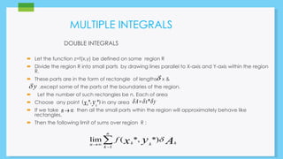
Fubini’s theorm
If f(x,y) is continuous throught the rectangular region
f ( x , y ) dA f ( x , y )
dxdy
f x y dA f x y dydx
&
d b
R c a
b d
( , ) ( , )
R a c
d b d b
f ( x , y ) dxdy [ f ( x , y ) dx ]
dy
c a c a](https://image.slidesharecdn.com/calculas-141127022342-conversion-gate02/85/multiple-intrigral-lit-8-320.jpg)
![MULTIPLE INTEGRAL
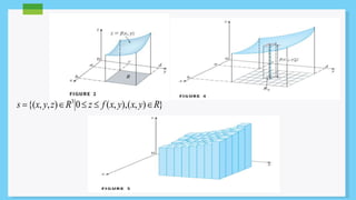
For example
2 1
(13xy)dxdy
1 0
2 2
x y
1
0
I x dy
1
3
[ ]
2
2
I dy
1
3
y
(1 )
2
2
2
1
3
y
y
[ ]
4
12 3
[2 1 ]
4 4
3
4
4](https://image.slidesharecdn.com/calculas-141127022342-conversion-gate02/85/multiple-intrigral-lit-9-320.jpg)

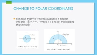
![CHANGE TO POLAR COORDINATES
To compute the double integral
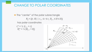
where R is a polar rectangle, we divide:
The interval [a, b] into m subintervals [ri–1, ri]
of equal width Δr = (b – a)/m.
The interval [α ,β] into n subintervals [θj–1, θi]
of equal width Δθ = (β – α)/n.](https://image.slidesharecdn.com/calculas-141127022342-conversion-gate02/85/multiple-intrigral-lit-13-320.jpg)


This document contains information about a calculus project completed by students of the Mechanical Engineering department at Laxmi Institute of Technology in Sarigam. It includes the names and student IDs of 13 students who participated in the project. The document covers topics in multiple integrals, including double integrals, Fubini's theorem, double integrals in polar coordinates, and triple integrals. Formulas and examples are provided for each topic.