This document provides an overview of mathematical formulae across various topics. It includes formulae for series such as arithmetic and geometric progressions. It also covers vector algebra, matrix algebra, vector calculus, complex variables, trigonometric functions, hyperbolic functions, limits, differentiation, integration, differential equations, calculus of variations, functions of several variables, Fourier series and transforms, Laplace transforms, numerical analysis, treatment of random errors, and statistics. Physical constants are also provided as a reference.

1. Mathematical Formula Handbook

2. Contents
Introduction. . . . . . . . . . . . . . . . . . . . . . . . . . . . . . . . . . . . . . . . . . . . . . . . . . . . . . . . . . . . . . . . . . . . . . . . . . . . . . . . . . . . . . . . . . . . 1
Bibliography; Physical Constants
1. Series. . . . . . . . . . . . . . . . . . . . . . . . . . . . . . . . . . . . . . . . . . . . . . . . . . . . . . . . . . . . . . . . . . . . . . . . . . . . . . . . . . . . . . . . . . . . . . . . . . . . 2
Arithmetic and Geometric progressions; Convergence of series: the ratio test;
Convergence of series: the comparison test; Binomial expansion; Taylor and Maclaurin Series;
Power series with real variables; Integer series; Plane wave expansion
2. Vector Algebra. . . . . . . . . . . . . . . . . . . . . . . . . . . . . . . . . . . . . . . . . . . . . . . . . . . . . . . . . . . . . . . . . . . . . . . . . . . . . . . . . . . . . . . . . 3
Scalar product; Equation of a line; Equation of a plane; Vector product; Scalar triple product;
Vector triple product; Non-orthogonal basis; Summation convention
3. Matrix Algebra . . . . . . . . . . . . . . . . . . . . . . . . . . . . . . . . . . . . . . . . . . . . . . . . . . . . . . . . . . . . . . . . . . . . . . . . . . . . . . . . . . . . . . . . 5
Unit matrices; Products; Transpose matrices; Inverse matrices; Determinants; 2×2 matrices;
Product rules; Orthogonal matrices; Solving sets of linear simultaneous equations; Hermitian matrices;
Eigenvalues and eigenvectors; Commutators; Hermitian algebra; Pauli spin matrices
4. Vector Calculus . . . . . . . . . . . . . . . . . . . . . . . . . . . . . . . . . . . . . . . . . . . . . . . . . . . . . . . . . . . . . . . . . . . . . . . . . . . . . . . . . . . . . . . . 7
Notation; Identities; Grad, Div, Curl and the Laplacian; Transformation of integrals
5. Complex Variables . . . . . . . . . . . . . . . . . . . . . . . . . . . . . . . . . . . . . . . . . . . . . . . . . . . . . . . . . . . . . . . . . . . . . . . . . . . . . . . . . . . . 9
Complex numbers; De Moivre’s theorem; Power series for complex variables.
6. Trigonometric Formulae . . . . . . . . . . . . . . . . . . . . . . . . . . . . . . . . . . . . . . . . . . . . . . . . . . . . . . . . . . . . . . . . . . . . . . . . . . . . 10
Relations between sides and angles of any plane triangle;
Relations between sides and angles of any spherical triangle
7. Hyperbolic Functions . . . . . . . . . . . . . . . . . . . . . . . . . . . . . . . . . . . . . . . . . . . . . . . . . . . . . . . . . . . . . . . . . . . . . . . . . . . . . . . 11
Relations of the functions; Inverse functions
8. Limits. . . . . . . . . . . . . . . . . . . . . . . . . . . . . . . . . . . . . . . . . . . . . . . . . . . . . . . . . . . . . . . . . . . . . . . . . . . . . . . . . . . . . . . . . . . . . . . . . . 12
9. Differentiation. . . . . . . . . . . . . . . . . . . . . . . . . . . . . . . . . . . . . . . . . . . . . . . . . . . . . . . . . . . . . . . . . . . . . . . . . . . . . . . . . . . . . . . . 13
10. Integration . . . . . . . . . . . . . . . . . . . . . . . . . . . . . . . . . . . . . . . . . . . . . . . . . . . . . . . . . . . . . . . . . . . . . . . . . . . . . . . . . . . . . . . . . . . . 13
Standard forms; Standard substitutions; Integration by parts; Differentiation of an integral;
Dirac δ-‘function’; Reduction formulae
11. Differential Equations . . . . . . . . . . . . . . . . . . . . . . . . . . . . . . . . . . . . . . . . . . . . . . . . . . . . . . . . . . . . . . . . . . . . . . . . . . . . . . . 16
Diffusion (conduction) equation; Wave equation; Legendre’s equation; Bessel’s equation;
Laplace’s equation; Spherical harmonics
12. Calculus of Variations . . . . . . . . . . . . . . . . . . . . . . . . . . . . . . . . . . . . . . . . . . . . . . . . . . . . . . . . . . . . . . . . . . . . . . . . . . . . . . . 17
13. Functions of Several Variables . . . . . . . . . . . . . . . . . . . . . . . . . . . . . . . . . . . . . . . . . . . . . . . . . . . . . . . . . . . . . . . . . . . . . 18
Taylor series for two variables; Stationary points; Changing variables: the chain rule;
Changing variables in surface and volume integrals – Jacobians
14. Fourier Series and Transforms . . . . . . . . . . . . . . . . . . . . . . . . . . . . . . . . . . . . . . . . . . . . . . . . . . . . . . . . . . . . . . . . . . . . . 19
Fourier series; Fourier series for other ranges; Fourier series for odd and even functions;
Complex form of Fourier series; Discrete Fourier series; Fourier transforms; Convolution theorem;
Parseval’s theorem; Fourier transforms in two dimensions; Fourier transforms in three dimensions
15. Laplace Transforms. . . . . . . . . . . . . . . . . . . . . . . . . . . . . . . . . . . . . . . . . . . . . . . . . . . . . . . . . . . . . . . . . . . . . . . . . . . . . . . . . . 23
16. Numerical Analysis . . . . . . . . . . . . . . . . . . . . . . . . . . . . . . . . . . . . . . . . . . . . . . . . . . . . . . . . . . . . . . . . . . . . . . . . . . . . . . . . . 24
Finding the zeros of equations; Numerical integration of differential equations;
Central difference notation; Approximating to derivatives; Interpolation: Everett’s formula;
Numerical evaluation of definite integrals
17. Treatment of Random Errors . . . . . . . . . . . . . . . . . . . . . . . . . . . . . . . . . . . . . . . . . . . . . . . . . . . . . . . . . . . . . . . . . . . . . . . 25
Range method; Combination of errors
18. Statistics . . . . . . . . . . . . . . . . . . . . . . . . . . . . . . . . . . . . . . . . . . . . . . . . . . . . . . . . . . . . . . . . . . . . . . . . . . . . . . . . . . . . . . . . . . . . . . . 26
Mean and Variance; Probability distributions; Weighted sums of random variables;
Statistics of a data sample x1, . . . , xn; Regression (least squares fitting)

3. Introduction
This Mathematical Formaulae handbook has been prepared in response to a request from the Physics Consultative
Committee, with the hope that it will be useful to those studying physics. It is to some extent modelled on a similar
document issued by the Department of Engineering, but obviously reflects the particular interests of physicists.
There was discussion as to whether it should also include physical formulae such as Maxwell’s equations, etc., but
a decision was taken against this, partly on the grounds that the book would become unduly bulky, but mainly
because, in its present form, clean copies can be made available to candidates in exams.
There has been wide consultation among the staff about the contents of this document, but inevitably some users
will seek in vain for a formula they feel strongly should be included. Please send suggestions for amendments to
the Secretary of the Teaching Committee, and they will be considered for incorporation in the next edition. The
Secretary will also be grateful to be informed of any (equally inevitable) errors which are found.
This book was compiled by Dr John Shakeshaft and typeset originally by Fergus Gallagher, and currently by
Dr Dave Green, using the TEX typesetting package.
Version 1.5 December 2005.
Bibliography
Abramowitz, M. & Stegun, I.A., Handbook of Mathematical Functions, Dover, 1965.
Gradshteyn, I.S. & Ryzhik, I.M., Table of Integrals, Series and Products, Academic Press, 1980.
Jahnke, E. & Emde, F., Tables of Functions, Dover, 1986.
Nordling, C. & ¨Osterman, J., Physics Handbook, Chartwell-Bratt, Bromley, 1980.
Speigel, M.R., Mathematical Handbook of Formulas and Tables.
(Schaum’s Outline Series, McGraw-Hill, 1968).
Physical Constants
Based on the “Review of Particle Properties”, Barnett et al., 1996, Physics Review D, 54, p1, and “The Fundamental
Physical Constants”, Cohen & Taylor, 1997, Physics Today, BG7. (The figures in parentheses give the 1-standard-
deviation uncertainties in the last digits.)
speed of light in a vacuum c 2·997 924 58 × 108 m s−1 (by definition)
permeability of a vacuum µ0 4π × 10−7 H m−1 (by definition)
permittivity of a vacuum 0 1/µ0c2 = 8·854 187 817 . . . × 10−12 F m−1
elementary charge e 1·602 177 33(49) × 10−19 C
Planck constant h 6·626 075 5(40) × 10−34 J s
h/2π ¯¯h 1·054 572 66(63) × 10−34 J s
Avogadro constant NA 6·022 136 7(36) × 1023 mol−1
unified atomic mass constant mu 1·660 540 2(10) × 10−27 kg
mass of electron me 9·109 389 7(54) × 10−31 kg
mass of proton mp 1·672 623 1(10) × 10−27 kg
Bohr magneton eh/4πme µB 9·274 015 4(31) × 10−24 J T−1
molar gas constant R 8·314 510(70) J K−1 mol−1
Boltzmann constant kB 1·380 658(12) × 10−23 J K−1
Stefan–Boltzmann constant σ 5·670 51(19) × 10−8 W m−2 K−4
gravitational constant G 6·672 59(85) × 10−11 N m2 kg−2
Other data
acceleration of free fall g 9·806 65 m s−2 (standard value at sea level)
1

4. 1. Series
Arithmetic and Geometric progressions
A.P. Sn = a + (a + d) + (a + 2d) + · · · + [a + (n − 1)d] =
n
2
[2a + (n − 1)d]
G.P. Sn = a + ar + ar2
+ · · · + arn−1
= a
1 − rn
1 − r
, S∞ =
a
1 − r
for |r| < 1
(These results also hold for complex series.)
Convergence of series: the ratio test
Sn = u1 + u2 + u3 + · · · + un converges as n → ∞ if lim
n→∞
un+1
un
< 1
Convergence of series: the comparison test
If each term in a series of positive terms is less than the corresponding term in a series known to be convergent,
then the given series is also convergent.
Binomial expansion
(1 + x)n
= 1 + nx +
n(n − 1)
2!
x2
+
n(n − 1)(n − 2)
3!
x3
+ · · ·
If n is a positive integer the series terminates and is valid for all x: the term in xr
is n
Crxr
or
n
r
where n
Cr ≡
n!
r!(n − r)!
is the number of different ways in which an unordered sample of r objects can be selected from a set of
n objects without replacement. When n is not a positive integer, the series does not terminate: the infinite series is
convergent for |x| < 1.
Taylor and Maclaurin Series
If y(x) is well-behaved in the vicinity of x = a then it has a Taylor series,
y(x) = y(a + u) = y(a) + u
dy
dx
+
u2
2!
d2
y
dx2
+
u3
3!
d3
y
dx3
+ · · ·
where u = x − a and the differential coefficients are evaluated at x = a. A Maclaurin series is a Taylor series with
a = 0,
y(x) = y(0) + x
dy
dx
+
x2
2!
d2
y
dx2
+
x3
3!
d3
y
dx3
+ · · ·
Power series with real variables
ex
= 1 + x +
x2
2!
+ · · · +
xn
n!
+ · · · valid for all x
ln(1 + x) = x −
x2
2
+
x3
3
+ · · · + (−1)n+1 xn
n
+ · · · valid for −1 < x ≤ 1
cos x =
eix
+ e−ix
2
= 1 −
x2
2!
+
x4
4!
−
x6
6!
+ · · · valid for all values of x
sin x =
eix
− e−ix
2i
= x −
x3
3!
+
x5
5!
+ · · · valid for all values of x
tan x = x +
1
3
x3
+
2
15
x5
+ · · · valid for −
π
2
< x <
π
2
tan−1
x = x −
x3
3
+
x5
5
− · · · valid for −1 ≤ x ≤ 1
sin−1
x = x +
1
2
x3
3
+
1.3
2.4
x5
5
+ · · · valid for −1 < x < 1
2

5. Integer series
N
∑
1
n = 1 + 2 + 3 + · · · + N =
N(N + 1)
2
N
∑
1
n2
= 12
+ 22
+ 32
+ · · · + N2
=
N(N + 1)(2N + 1)
6
N
∑
1
n3
= 13
+ 23
+ 33
+ · · · + N3
= [1 + 2 + 3 + · · · N]2
=
N2
(N + 1)2
4
∞
∑
1
(−1)n+1
n
= 1 −
1
2
+
1
3
−
1
4
+ · · · = ln 2 [see expansion of ln(1 + x)]
∞
∑
1
(−1)n+1
2n − 1
= 1 −
1
3
+
1
5
−
1
7
+ · · · =
π
4
[see expansion of tan−1
x]
∞
∑
1
1
n2
= 1 +
1
4
+
1
9
+
1
16
+ · · · =
π2
6
N
∑
1
n(n + 1)(n + 2) = 1.2.3 + 2.3.4 + · · · + N(N + 1)(N + 2) =
N(N + 1)(N + 2)(N + 3)
4
This last result is a special case of the more general formula,
N
∑
1
n(n + 1)(n + 2) . . . (n + r) =
N(N + 1)(N + 2) . . . (N + r)(N + r + 1)
r + 2
.
Plane wave expansion
exp(ikz) = exp(ikr cosθ) =
∞
∑
l=0
(2l + 1)il
jl(kr)Pl(cosθ),
where Pl(cosθ) are Legendre polynomials (see section 11) and jl(kr) are spherical Bessel functions, defined by
jl(ρ) =
π
2ρ
Jl+1/2
(ρ), with Jl(x) the Bessel function of order l (see section 11).
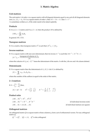
2. Vector Algebra
If i, j, k are orthonormal vectors and A = Axi + Ay j + Azk then |A|2
= A2
x + A2
y + A2
z. [Orthonormal vectors ≡
orthogonal unit vectors.]
Scalar product
A · B = |A| |B| cosθ where θ is the angle between the vectors
= AxBx + AyBy + AzBz = [ Ax Ay Az ]


Bx
By
Bz


Scalar multiplication is commutative: A · B = B · A.
Equation of a line
A point r ≡ (x, y, z) lies on a line passing through a point a and parallel to vector b if
r = a + λb
with λ a real number.
3

6. Equation of a plane
A point r ≡ (x, y, z) is on a plane if either
(a) r · d = |d|, where d is the normal from the origin to the plane, or
(b)
x
X
+
y
Y
+
z
Z
= 1 where X, Y, Z are the intercepts on the axes.
Vector product
A×B = n |A| |B| sinθ, whereθ is the angle between the vectors and n is a unit vector normal to the plane containing
A and B in the direction for which A, B, n form a right-handed set of axes.
A × B in determinant form
i j k
Ax Ay Az
Bx By Bz
A × B in matrix form


0 −Az Ay
Az 0 −Ax
−Ay Ax 0




Bx
By
Bz


Vector multiplication is not commutative: A × B = −B × A.
Scalar triple product
A × B · C = A · B × C =
Ax Ay Az
Bx By Bz
Cx Cy Cz
= −A × C · B, etc.
Vector triple product
A × (B × C) = (A · C)B − (A · B)C, (A × B) × C = (A · C)B − (B · C)A
Non-orthogonal basis
A = A1e1 + A2e2 + A3e3
A1 = · A where =
e2 × e3
e1 · (e2 × e3)
Similarly for A2 and A3.
Summation convention
a = aiei implies summation over i = 1 . . . 3
a · b = aibi
(a × b)i = εijkajbk where ε123 = 1; εijk = −εikj
εijkεklm = δilδjm − δimδjl
4

7. 3. Matrix Algebra
Unit matrices
The unit matrix I of order n is a square matrix with all diagonal elements equal to one and all off-diagonal elements
zero, i.e., (I)ij = δij. If A is a square matrix of order n, then AI = IA = A. Also I = I−1
.
I is sometimes written as In if the order needs to be stated explicitly.
Products
If A is a (n × l) matrix and B is a (l × m) then the product AB is defined by
(AB)ij =
l
∑
k=1
AikBkj
In general AB = BA.
Transpose matrices
If A is a matrix, then transpose matrix AT
is such that (AT
)ij = (A)ji.
Inverse matrices
If A is a square matrix with non-zero determinant, then its inverse A−1
is such that AA−1
= A−1
A = I.
(A−1
)ij =
transpose of cofactor of Aij
|A|
where the cofactor of Aij is (−1)i+j
times the determinant of the matrix A with the j-th row and i-th column deleted.
Determinants
If A is a square matrix then the determinant of A, |A| (≡ det A) is defined by
|A| = ∑
i,j,k,...
ijk...A1i A2j A3k . . .
where the number of the suffixes is equal to the order of the matrix.
2×2 matrices
If A =
a b
c d
then,
|A| = ad − bc AT
=
a c
b d
A−1
=
1
|A|
d −b
−c a
Product rules
(AB . . . N)T
= NT
. . . BT
AT
(AB . . . N)−1
= N−1
. . . B−1
A−1
(if individual inverses exist)
|AB . . . N| = |A| |B| . . . |N| (if individual matrices are square)
Orthogonal matrices
An orthogonal matrix Q is a square matrix whose columns qi form a set of orthonormal vectors. For any orthogonal
matrix Q,
Q−1
= QT
, |Q| = ±1, QT
is also orthogonal.
5

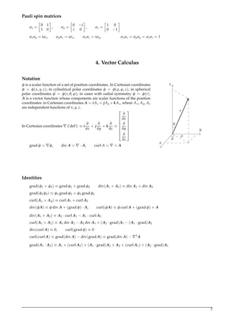
8. Solving sets of linear simultaneous equations
If A is square then Ax = b has a unique solution x = A−1
b if A−1
exists, i.e., if |A| = 0.
If A is square then Ax = 0 has a non-trivial solution if and only if |A| = 0.
An over-constrained set of equations Ax = b is one in which A has m rows and n columns, where m (the number
of equations) is greater than n (the number of variables). The best solution x (in the sense that it minimizes the
error |Ax − b|) is the solution of the n equations AT
Ax = AT
b. If the columns of A are orthonormal vectors then
x = AT
b.
Hermitian matrices
The Hermitian conjugate of A is A† = (A∗
)T
, where A∗
is a matrix each of whose components is the complex
conjugate of the corresponding components of A. If A = A† then A is called a Hermitian matrix.
Eigenvalues and eigenvectors
The n eigenvalues λi and eigenvectors ui of an n × n matrix A are the solutions of the equation Au = λu. The
eigenvalues are the zeros of the polynomial of degree n, Pn(λ) = |A − λI|. If A is Hermitian then the eigenvalues
λi are real and the eigenvectors ui are mutually orthogonal. |A − λI| = 0 is called the characteristic equation of the
matrix A.
Tr A = ∑
i
λi, also |A| = ∏
i
λi.
If S is a symmetric matrix, Λ is the diagonal matrix whose diagonal elements are the eigenvalues of S, and U is the
matrix whose columns are the normalized eigenvectors of A, then
UT
SU = Λ and S = UΛUT
.
If x is an approximation to an eigenvector of A then xT
Ax/(xT
x) (Rayleigh’s quotient) is an approximation to the
corresponding eigenvalue.
Commutators
[A, B] ≡ AB − BA
[A, B] = −[B, A]
[A, B]† = [B†, A†]
[A + B, C] = [A, C] + [B, C]
[AB, C] = A[B, C] + [A, C]B
[A, [B, C]] + [B, [C, A]] + [C, [A, B]] = 0
Hermitian algebra
b† = (b∗
1, b∗
2, . . .)
Matrix form Operator form Bra-ket form
Hermiticity b∗
· A · c = (A · b)∗
· c
Z
ψ∗
Oφ =
Z
(Oψ)∗
φ ψ|O|φ
Eigenvalues, λ real Aui = λ(i)ui Oψi = λ(i)ψi O |i = λi |i
Orthogonality ui · uj = 0
Z
ψ∗
i ψj = 0 i|j = 0 (i = j)
Completeness b = ∑
i
ui(ui · b) φ = ∑
i
ψi
Z
ψ∗
i φ φ = ∑
i
|i i|φ
Rayleigh–Ritz
Lowest eigenvalue λ0 ≤
b∗
· A · b
b∗
· b
λ0 ≤
Z
ψ∗
Oψ
Z
ψ∗
ψ
ψ|O|ψ
ψ|ψ
6

9. Pauli spin matrices
σx =
0 1
1 0
, σy =
0 −i
i 0
, σz =
1 0
0 −1
σxσy = iσz, σyσz = iσx, σzσx = iσy, σxσx = σyσy = σzσz = I
4. Vector Calculus
Notation
φ is a scalar function of a set of position coordinates. In Cartesian coordinates
φ = φ(x, y, z); in cylindrical polar coordinates φ = φ(ρ,ϕ, z); in spherical
polar coordinates φ = φ(r,θ,ϕ); in cases with radial symmetry φ = φ(r).
A is a vector function whose components are scalar functions of the position
coordinates: in Cartesian coordinates A = iAx + jAy + kAz, where Ax, Ay, Az
are independent functions of x, y, z.
In Cartesian coordinates (‘del’) ≡ i
∂
∂x
+ j
∂
∂y
+ k
∂
∂z
≡









∂
∂x
∂
∂y
∂
∂z









gradφ = φ, div A = · A, curl A = × A
Identities
grad(φ1 + φ2) ≡ gradφ1 + gradφ2 div(A1 + A2) ≡ div A1 + div A2
grad(φ1φ2) ≡ φ1 gradφ2 + φ2 gradφ1
curl(A + A) ≡ curl A1 + curl A2
div(φA) ≡ φ div A + (gradφ) · A, curl(φA) ≡ φ curl A + (gradφ) × A
div(A1 × A2) ≡ A2 · curl A1 − A1 · curl A2
curl(A1 × A2) ≡ A1 div A2 − A2 div A1 + (A2 · grad)A1 − (A1 · grad)A2
div(curl A) ≡ 0, curl(gradφ) ≡ 0
curl(curl A) ≡ grad(div A) − div(grad A) ≡ grad(div A) − 2
A
grad(A1 · A2) ≡ A1 × (curl A2) + (A1 · grad)A2 + A2 × (curl A1) + (A2 · grad)A1
7

10. Grad, Div, Curl and the Laplacian
Cartesian Coordinates Cylindrical Coordinates Spherical Coordinates
Conversion to
Cartesian
Coordinates
x = ρ cosϕ y = ρ sinϕ z = z
x = r cosϕ sinθ y = r sinϕ sinθ
z = r cosθ
Vector A Axi + Ay j + Azk Aρρ + Aϕϕ + Azz Arr + Aθθ + Aϕϕ
Gradient φ
∂φ
∂x
i +
∂φ
∂y
j +
∂φ
∂z
k
∂φ
∂ρ
ρ +
1
ρ
∂φ
∂ϕ
ϕ +
∂φ
∂z
z
∂φ
∂r
r +
1
r
∂φ
∂θ
θ +
1
r sinθ
∂φ
∂ϕ
ϕ
Divergence
· A
∂Ax
∂x
+
∂Ay
∂y
+
∂Az
∂z
1
ρ
∂(ρAρ)
∂ρ
+
1
ρ
∂Aϕ
∂ϕ
+
∂Az
∂z
1
r2
∂(r2
Ar)
∂r
+
1
r sinθ
∂Aθ sinθ
∂θ
+
1
r sinθ
∂Aϕ
∂ϕ
Curl × A
i j k
∂
∂x
∂
∂y
∂
∂z
Ax Ay Az
1
ρ
ρ ϕ
1
ρ
z
∂
∂ρ
∂
∂ϕ
∂
∂z
Aρ ρAϕ Az
1
r2
sinθ
r
1
r sinθ
θ
1
r
ϕ
∂
∂r
∂
∂θ
∂
∂ϕ
Ar rAθ rAϕ sinθ
Laplacian
2
φ
∂2
φ
∂x2
+
∂2
φ
∂y2
+
∂2
φ
∂z2
1
ρ
∂
∂ρ
ρ
∂φ
∂ρ
+
1
ρ2
∂2
φ
∂ϕ2
+
∂2
φ
∂z2
1
r2
∂
∂r
r2 ∂φ
∂r
+
1
r2
sinθ
∂
∂θ
sinθ
∂φ
∂θ
+
1
r2
sin2
θ
∂2
φ
∂ϕ2
Transformation of integrals
L = the distance along some curve ‘C’ in space and is measured from some fixed point.
S = a surface area
τ = a volume contained by a specified surface
t = the unit tangent to C at the point P
n = the unit outward pointing normal
A = some vector function
dL = the vector element of curve (= t dL)
dS = the vector element of surface (= n dS)
Then
Z
C
A · t dL =
Z
C
A · dL
and when A = φ
Z
C
( φ) · dL =
Z
C
dφ
Gauss’s Theorem (Divergence Theorem)
When S defines a closed region having a volume τ
Z
τ
( · A) dτ =
Z
S
(A · n) dS =
Z
S
A · dS
also
Z
τ
( φ) dτ =
Z
S
φ dS
Z
τ
( × A) dτ =
Z
S
(n × A) dS
8

11. Stokes’s Theorem
When C is closed and bounds the open surface S,
Z
S
( × A) · dS =
Z
C
A · dL
also
Z
S
(n × φ) dS =
Z
C
φ dL
Green’s Theorem
Z
S
ψ φ · dS =
Z
τ
· (ψ φ) dτ
=
Z
τ
ψ 2
φ + ( ψ) · ( φ) dτ
Green’s Second Theorem
Z
τ
(ψ 2
φ − φ 2
ψ) dτ =
Z
S
[ψ( φ) − φ( ψ)] · dS
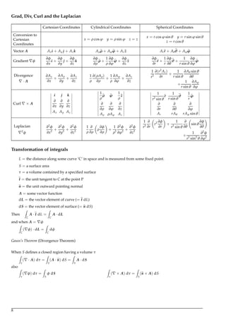
5. Complex Variables
Complex numbers
The complex number z = x + iy = r(cosθ + i sinθ) = r ei(θ+2nπ)
, where i2
= −1 and n is an arbitrary integer. The
real quantity r is the modulus of z and the angle θ is the argument of z. The complex conjugate of z is z∗
= x − iy =
r(cosθ − i sinθ) = r e−iθ
; zz∗
= |z|2
= x2
+ y2
De Moivre’s theorem
(cosθ + i sinθ)n
= einθ
= cos nθ + i sin nθ
Power series for complex variables.
ez
= 1 + z +
z2
2!
+ · · · +
zn
n!
+ · · · convergent for all finite z
sin z = z −
z3
3!
+
z5
5!
− · · · convergent for all finite z
cos z = 1 −
z2
2!
+
z4
4!
− · · · convergent for all finite z
ln(1 + z) = z −
z2
2
+
z3
3
− · · · principal value of ln(1 + z)
This last series converges both on and within the circle |z| = 1 except at the point z = −1.
tan−1
z = z −
z3
3
+
z5
5
− · · ·
This last series converges both on and within the circle |z| = 1 except at the points z = ±i.
(1 + z)n
= 1 + nz +
n(n − 1)
2!
z2
+
n(n − 1)(n − 2)
3!
z3
+ · · ·
This last series converges both on and within the circle |z| = 1 except at the point z = −1.
9

12. 6. Trigonometric Formulae
cos2
A + sin2
A = 1 sec2
A − tan2
A = 1 cosec2
A − cot2
A = 1
sin 2A = 2 sin A cos A cos 2A = cos2
A − sin2
A tan 2A =
2 tan A
1 − tan2
A
.
sin(A ± B) = sin A cos B ± cos A sin B cos A cos B =
cos(A + B) + cos(A − B)
2
cos(A ± B) = cos A cos B sin A sin B sin A sin B =
cos(A − B) − cos(A + B)
2
tan(A ± B) =
tan A ± tan B
1 tan A tan B
sin A cos B =
sin(A + B) + sin(A − B)
2
sin A + sin B = 2 sin
A + B
2
cos
A − B
2
sin A − sin B = 2 cos
A + B
2
sin
A − B
2
cos A + cos B = 2 cos
A + B
2
cos
A − B
2
cos A − cos B = −2 sin
A + B
2
sin
A − B
2
cos2
A =
1 + cos 2A
2
sin2
A =
1 − cos 2A
2
cos3
A =
3 cos A + cos 3A
4
sin3
A =
3 sin A − sin 3A
4
Relations between sides and angles of any plane triangle
In a plane triangle with angles A, B, and C and sides opposite a, b, and c respectively,
a
sin A
=
b
sin B
=
c
sin C
= diameter of circumscribed circle.
a2
= b2
+ c2
− 2bc cos A
a = b cos C + c cos B
cos A =
b2
+ c2
− a2
2bc
tan
A − B
2
=
a − b
a + b
cot
C
2
area =
1
2
ab sin C =
1
2
bc sin A =
1
2
ca sin B = s(s − a)(s − b)(s − c), where s =
1
2
(a + b + c)
Relations between sides and angles of any spherical triangle
In a spherical triangle with angles A, B, and C and sides opposite a, b, and c respectively,
sin a
sin A
=
sin b
sin B
=
sin c
sin C
cos a = cos b cos c + sin b sin c cos A
cos A = − cos B cos C + sin B sin C cos a
10

13. 7. Hyperbolic Functions
cosh x =
1
2
( ex
+ e−x
) = 1 +
x2
2!
+
x4
4!
+ · · · valid for all x
sinh x =
1
2
( ex
− e−x
) = x +
x3
3!
+
x5
5!
+ · · · valid for all x
cosh ix = cos x cos ix = cosh x
sinh ix = i sin x sin ix = i sinh x
tanh x =
sinh x
cosh x
sech x =
1
cosh x
coth x =
cosh x
sinh x
cosech x =
1
sinh x
cosh2
x − sinh2
x = 1
For large positive x:
cosh x ≈ sinh x →
ex
2
tanh x → 1
For large negative x:
cosh x ≈ − sinh x →
e−x
2
tanh x → −1
Relations of the functions
sinh x = − sinh(−x) sech x = sech(−x)
cosh x = cosh(−x) cosech x = − cosech(−x)
tanh x = − tanh(−x) coth x = − coth(−x)
sinh x =
2 tanh (x/2)
1 − tanh2
(x/2)
=
tanh x
1 − tanh2
x
cosh x =
1 + tanh2
(x/2)
1 − tanh2
(x/2)
=
1
1 − tanh2
x
tanh x = 1 − sech2
x sech x = 1 − tanh2
x
coth x = cosech2
x + 1 cosech x = coth2
x − 1
sinh(x/2) =
cosh x − 1
2
cosh(x/2) =
cosh x + 1
2
tanh(x/2) =
cosh x − 1
sinh x
=
sinh x
cosh x + 1
sinh(2x) = 2 sinh x cosh x tanh(2x) =
2 tanh x
1 + tanh2
x
cosh(2x) = cosh2
x + sinh2
x = 2 cosh2
x − 1 = 1 + 2 sinh2
x
sinh(3x) = 3 sinh x + 4 sinh3
x cosh 3x = 4 cosh3
x − 3 cosh x
tanh(3x) =
3 tanh x + tanh3
x
1 + 3 tanh2
x
11

14. sinh(x ± y) = sinh x cosh y ± cosh x sinh y
cosh(x ± y) = cosh x cosh y ± sinh x sinh y
tanh(x ± y) =
tanh x ± tanh y
1 ± tanh x tanh y
sinh x + sinh y = 2 sinh
1
2
(x + y) cosh
1
2
(x − y) cosh x + cosh y = 2 cosh
1
2
(x + y) cosh
1
2
(x − y)
sinh x − sinh y = 2 cosh
1
2
(x + y) sinh
1
2
(x − y) cosh x − cosh y = 2 sinh
1
2
(x + y) sinh
1
2
(x − y)
sinh x ± cosh x =
1 ± tanh (x/2)
1 tanh(x/2)
= e±x
tanh x ± tanh y =
sinh(x ± y)
cosh x cosh y
coth x ± coth y = ±
sinh(x ± y)
sinh x sinh y
Inverse functions
sinh−1 x
a
= ln
x + x2 + a2
a
for −∞ < x < ∞
cosh−1 x
a
= ln
x + x2 − a2
a
for x ≥ a
tanh−1 x
a
=
1
2
ln
a + x
a − x
for x2
< a2
coth−1 x
a
=
1
2
ln
x + a
x − a
for x2
> a2
sech−1 x
a
= ln

 a
x
+
a2
x2
− 1

 for 0 < x ≤ a
cosech−1 x
a
= ln

 a
x
+
a2
x2
+ 1

 for x = 0
8. Limits
nc
xn
→ 0 as n → ∞ if |x| < 1 (any fixed c)
xn
/n! → 0 as n → ∞ (any fixed x)
(1 + x/n)n
→ ex
as n → ∞, x ln x → 0 as x → 0
If f (a) = g(a) = 0 then lim
x→a
f (x)
g(x)
=
f (a)
g (a)
(l’Hˆopital’s rule)
12

15. 9. Differentiation
(uv) = u v + uv ,
u
v
=
u v − uv
v2
(uv)(n)
= u(n)
v + nu(n−1)
v(1)
+ · · · + n
Cru(n−r)
v(r)
+ · · · + uv(n)
Leibniz Theorem
where n
Cr ≡
n
r
=
n!
r!(n − r)!
d
dx
(sin x) = cos x
d
dx
(sinh x) = cosh x
d
dx
(cos x) = − sin x
d
dx
(cosh x) = sinh x
d
dx
(tan x) = sec2
x
d
dx
(tanh x) = sech2
x
d
dx
(sec x) = sec x tan x
d
dx
(sech x) = − sech x tanh x
d
dx
(cot x) = − cosec2
x
d
dx
(coth x) = − cosech2
x
d
dx
(cosec x) = − cosec x cot x
d
dx
(cosech x) = − cosech x coth x
10. Integration
Standard forms
Z
xn
dx =
xn+1
n + 1
+ c for n = −1
Z
1
x
dx = ln x + c
Z
ln x dx = x(ln x − 1) + c
Z
eax
dx =
1
a
eax
+ c
Z
x eax
dx = eax x
a
−
1
a2
+ c
Z
x ln x dx =
x2
2
ln x −
1
2
+ c
Z
1
a2
+ x2
dx =
1
a
tan−1 x
a
+ c
Z
1
a2
− x2
dx =
1
a
tanh−1 x
a
+ c =
1
2a
ln
a + x
a − x
+ c for x2
< a2
Z
1
x2
− a2
dx = −
1
a
coth−1 x
a
+ c =
1
2a
ln
x − a
x + a
+ c for x2
> a2
Z
x
(x2
± a2
)n
dx =
−1
2(n − 1)
1
(x2
± a2
)n−1
+ c for n = 1
Z
x
x2
± a2
dx =
1
2
ln(x2
± a2
) + c
Z
1
a2 − x2
dx = sin−1 x
a
+ c
Z
1
x2 ± a2
dx = ln x + x2 ± a2 + c
Z
x
x2 ± a2
dx = x2 ± a2 + c
Z
a2 − x2 dx =
1
2
x a2 − x2 + a2
sin−1 x
a
+ c
13

16. Z ∞
0
1
(1 + x)xp dx = π cosec pπ for p < 1
Z ∞
0
cos(x2
) dx =
Z ∞
0
sin(x2
) dx =
1
2
π
2
Z ∞
−∞
exp(−x2
/2σ2
) dx = σ
√
2π
Z ∞
−∞
xn
exp(−x2
/2σ2
) dx =



1 × 3 × 5 × · · · (n − 1)σn+1
√
2π
0
for n ≥ 2 and even
for n ≥ 1 and odd
Z
sin x dx = − cos x + c
Z
sinh x dx = cosh x + c
Z
cos x dx = sin x + c
Z
cosh x dx = sinh x + c
Z
tan x dx = − ln(cos x) + c
Z
tanh x dx = ln(cosh x) + c
Z
cosec x dx = ln(cosec x − cot x) + c
Z
cosech x dx = ln [tanh(x/2)] + c
Z
sec x dx = ln(sec x + tan x) + c
Z
sech x dx = 2 tan−1
( ex
) + c
Z
cot x dx = ln(sin x) + c
Z
coth x dx = ln(sinh x) + c
Z
sin mx sin nx dx =
sin(m − n)x
2(m − n)
−
sin(m + n)x
2(m + n)
+ c if m2
= n2
Z
cos mx cos nx dx =
sin(m − n)x
2(m − n)
+
sin(m + n)x
2(m + n)
+ c if m2
= n2
Standard substitutions
If the integrand is a function of: substitute:
(a2
− x2
) or a2 − x2 x = a sinθ or x = a cosθ
(x2
+ a2
) or x2 + a2 x = a tanθ or x = a sinhθ
(x2
− a2
) or x2 − a2 x = a secθ or x = a coshθ
If the integrand is a rational function of sin x or cos x or both, substitute t = tan(x/2) and use the results:
sin x =
2t
1 + t2
cos x =
1 − t2
1 + t2
dx =
2 dt
1 + t2
.
If the integrand is of the form: substitute:
Z
dx
(ax + b) px + q
px + q = u2
Z
dx
(ax + b) px2 + qx + r
ax + b =
1
u
.
14

17. Integration by parts
Z b
a
u dv = uv
b
a
−
Z b
a
v du
Differentiation of an integral
If f (x,α) is a function of x containing a parameter α and the limits of integration a and b are functions of α then
d
dα
Z b(α)
a(α)
f (x,α) dx = f (b,α)
db
dα
− f (a,α)
da
dα
+
Z b(α)
a(α)
∂
∂α
f (x,α) dx.
Special case,
d
dx
Z x
a
f (y) dy = f (x).
Dirac δ-‘function’
δ(t − τ) =
1
2π
Z ∞
−∞
exp[iω(t − τ)] dω.
If f (t) is an arbitrary function of t then
Z ∞
−∞
δ(t − τ) f (t) dt = f (τ).
δ(t) = 0 if t = 0, also
Z ∞
−∞
δ(t) dt = 1
Reduction formulae
Factorials
n! = n(n − 1)(n − 2) . . . 1, 0! = 1.
Stirling’s formula for large n: ln(n!) ≈ n ln n − n.
For any p > −1,
Z ∞
0
xp
e−x
dx = p
Z ∞
0
xp−1
e−x
dx = p!. (−1/2)! =
√
π, (1/2)! =
√
π/2, etc.
For any p, q > −1,
Z 1
0
xp
(1 − x)q
dx =
p!q!
(p + q + 1)!
.
Trigonometrical
If m, n are integers,
Z π/2
0
sinm
θ cosn
θ dθ =
m − 1
m + n
Z π/2
0
sinm−2
θ cosn
θ dθ =
n − 1
m + n
Z π/2
0
sinm
θ cosn−2
θ dθ
and can therefore be reduced eventually to one of the following integrals
Z π/2
0
sinθ cosθ dθ =
1
2
,
Z π/2
0
sinθ dθ = 1,
Z π/2
0
cosθ dθ = 1,
Z π/2
0
dθ =
π
2
.
Other
If In =
Z ∞
0
xn
exp(−αx2
) dx then In =
(n − 1)
2α
In−2, I0 =
1
2
π
α
, I1 =
1
2α
.
15

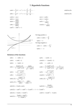
18. 11. Differential Equations
Diffusion (conduction) equation
∂ψ
∂t
= κ 2
ψ
Wave equation
2
ψ =
1
c2
∂2
ψ
∂t2
Legendre’s equation
(1 − x2
)
d2
y
dx2
− 2x
dy
dx
+ l(l + 1)y = 0,
solutions of which are Legendre polynomials Pl(x), where Pl(x) =
1
2l
l!
d
dx
l
x2
− 1
l
, Rodrigues’ formula so
P0(x) = 1, P1(x) = x, P2(x) =
1
2
(3x2
− 1) etc.
Recursion relation
Pl(x) =
1
l
[(2l − 1)xPl−1(x) − (l − 1)Pl−2(x)]
Orthogonality
Z 1
−1
Pl(x)Pl (x) dx =
2
2l + 1
δll
Bessel’s equation
x2 d2
y
dx2
+ x
dy
dx
+ (x2
− m2
)y = 0,
solutions of which are Bessel functions Jm(x) of order m.
Series form of Bessel functions of the first kind
Jm(x) =
∞
∑
k=0
(−1)k
(x/2)m+2k
k!(m + k)!
(integer m).
The same general form holds for non-integer m > 0.
16

19. Laplace’s equation
2
u = 0
If expressed in two-dimensional polar coordinates (see section 4), a solution is
u(ρ,ϕ) = Aρn
+ Bρ−n
C exp(inϕ) + D exp(−inϕ)
where A, B, C, D are constants and n is a real integer.
If expressed in three-dimensional polar coordinates (see section 4) a solution is
u(r,θ,ϕ) = Arl
+ Br−(l+1)
Pm
l C sin mϕ + D cos mϕ
where l and m are integers with l ≥ |m| ≥ 0; A, B, C, D are constants;
Pm
l (cosθ) = sin|m|
θ
d
d(cosθ)
|m|
Pl(cosθ)
is the associated Legendre polynomial.
P0
l (1) = 1.
If expressed in cylindrical polar coordinates (see section 4), a solution is
u(ρ,ϕ, z) = Jm(nρ) A cos mϕ + B sin mϕ C exp(nz) + D exp(−nz)
where m and n are integers; A, B, C, D are constants.
Spherical harmonics
The normalized solutions Ym
l (θ,ϕ) of the equation
1
sinθ
∂
∂θ
sinθ
∂
∂θ
+
1
sin2
θ
∂2
∂ϕ2
Ym
l + l(l + 1)Ym
l = 0
are called spherical harmonics, and have values given by
Ym
l (θ,ϕ) =
2l + 1
4π
(l − |m|)!
(l + |m|)!
Pm
l (cosθ) eimϕ
× (−1)m
for m ≥ 0
1 for m < 0
i.e., Y0
0 =
1
4π
, Y0
1 =
3
4π
cosθ, Y±1
1 =
3
8π
sinθ e±iϕ
, etc.
Orthogonality
Z
4π
Y∗m
l Ym
l dΩ = δll δmm
12. Calculus of Variations
The condition for I =
Z b
a
F(y, y , x) dx to have a stationary value is
∂F
∂y
=
d
dx
∂F
∂y
, where y =
dy
dx
. This is the
Euler–Lagrange equation.
17

20. 13. Functions of Several Variables
If φ = f (x, y, z, . . .) then
∂φ
∂x
implies differentiation with respect to x keeping y, z, . . . constant.
dφ =
∂φ
∂x
dx +
∂φ
∂y
dy +
∂φ
∂z
dz + · · · and δφ ≈
∂φ
∂x
δx +
∂φ
∂y
δy +
∂φ
∂z
δz + · · ·
where x, y, z, . . . are independent variables.
∂φ
∂x
is also written as
∂φ
∂x y,...
or
∂φ
∂x y,...
when the variables kept
constant need to be stated explicitly.
If φ is a well-behaved function then
∂2
φ
∂x ∂y
=
∂2
φ
∂y ∂x
etc.
If φ = f (x, y),
∂φ
∂x y
=
1
∂x
∂φ y
,
∂φ
∂x y
∂x
∂y φ
∂y
∂φ x
= −1.
Taylor series for two variables
If φ(x, y) is well-behaved in the vicinity of x = a, y = b then it has a Taylor series
φ(x, y) = φ(a + u, b + v) = φ(a, b) + u
∂φ
∂x
+ v
∂φ
∂y
+
1
2!
u2 ∂2
φ
∂x2
+ 2uv
∂2
φ
∂x ∂y
+ v2 ∂2
φ
∂y2
+ · · ·
where x = a + u, y = b + v and the differential coefficients are evaluated at x = a, y = b
Stationary points
A function φ = f (x, y) has a stationary point when
∂φ
∂x
=
∂φ
∂y
= 0. Unless
∂2
φ
∂x2
=
∂2
φ
∂y2
=
∂2
φ
∂x ∂y
= 0, the following
conditions determine whether it is a minimum, a maximum or a saddle point.
Minimum:
∂2
φ
∂x2
> 0, or
∂2
φ
∂y2
> 0,
Maximum:
∂2
φ
∂x2
< 0, or
∂2
φ
∂y2
< 0,



and
∂2
φ
∂x2
∂2
φ
∂y2
>
∂2
φ
∂x ∂y
2
Saddle point:
∂2
φ
∂x2
∂2
φ
∂y2
<
∂2
φ
∂x ∂y
2
If
∂2
φ
∂x2
=
∂2
φ
∂y2
=
∂2
φ
∂x ∂y
= 0 the character of the turning point is determined by the next higher derivative.
Changing variables: the chain rule
If φ = f (x, y, . . .) and the variables x, y, . . . are functions of independent variables u, v, . . . then
∂φ
∂u
=
∂φ
∂x
∂x
∂u
+
∂φ
∂y
∂y
∂u
+ · · ·
∂φ
∂v
=
∂φ
∂x
∂x
∂v
+
∂φ
∂y
∂y
∂v
+ · · ·
etc.
18

21. Changing variables in surface and volume integrals – Jacobians
If an area A in the x, y plane maps into an area A in the u, v plane then
Z
A
f (x, y) dx dy =
Z
A
f (u, v)J du dv where J =
∂x
∂u
∂x
∂v
∂y
∂u
∂y
∂v
The Jacobian J is also written as
∂(x, y)
∂(u, v)
. The corresponding formula for volume integrals is
Z
V
f (x, y, z) dx dy dz =
Z
V
f (u, v, w)J du dv dw where now J =
∂x
∂u
∂x
∂v
∂x
∂w
∂y
∂u
∂y
∂v
∂y
∂w
∂z
∂u
∂z
∂v
∂z
∂w
14. Fourier Series and Transforms
Fourier series
If y(x) is a function defined in the range −π ≤ x ≤ π then
y(x) ≈ c0 +
M
∑
m=1
cm cos mx +
M
∑
m=1
sm sin mx
where the coefficients are
c0 =
1
2π
Z π
−π
y(x) dx
cm =
1
π
Z π
−π
y(x) cos mx dx (m = 1, . . . , M)
sm =
1
π
Z π
−π
y(x) sin mx dx (m = 1, . . . , M )
with convergence to y(x) as M, M → ∞ for all points where y(x) is continuous.
Fourier series for other ranges
Variable t, range 0 ≤ t ≤ T, (i.e., a periodic function of time with period T, frequency ω = 2π/T).
y(t) ≈ c0 + ∑cm cos mωt + ∑sm sin mωt
where
c0 =
ω
2π
Z T
0
y(t) dt, cm =
ω
π
Z T
0
y(t) cos mωt dt, sm =
ω
π
Z T
0
y(t) sin mωt dt.
Variable x, range 0 ≤ x ≤ L,
y(x) ≈ c0 + ∑cm cos
2mπx
L
+ ∑sm sin
2mπx
L
where
c0 =
1
L
Z L
0
y(x) dx, cm =
2
L
Z L
0
y(x) cos
2mπx
L
dx, sm =
2
L
Z L
0
y(x) sin
2mπx
L
dx.
19

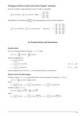
22. Fourier series for odd and even functions
If y(x) is an odd (anti-symmetric) function [i.e., y(−x) = −y(x)] defined in the range −π ≤ x ≤ π, then only
sines are required in the Fourier series and sm =
2
π
Z π
0
y(x) sin mx dx. If, in addition, y(x) is symmetric about
x = π/2, then the coefficients sm are given by sm = 0 (for m even), sm =
4
π
Z π/2
0
y(x) sin mx dx (for m odd). If
y(x) is an even (symmetric) function [i.e., y(−x) = y(x)] defined in the range −π ≤ x ≤ π, then only constant
and cosine terms are required in the Fourier series and c0 =
1
π
Z π
0
y(x) dx, cm =
2
π
Z π
0
y(x) cos mx dx. If, in
addition, y(x) is anti-symmetric about x =
π
2
, then c0 = 0 and the coefficients cm are given by cm = 0 (for m even),
cm =
4
π
Z π/2
0
y(x) cos mx dx (for m odd).
[These results also apply to Fourier series with more general ranges provided appropriate changes are made to the
limits of integration.]
Complex form of Fourier series
If y(x) is a function defined in the range −π ≤ x ≤ π then
y(x) ≈
M
∑
−M
Cm eimx
, Cm =
1
2π
Z π
−π
y(x) e−imx
dx
with m taking all integer values in the range ±M. This approximation converges to y(x) as M → ∞ under the same
conditions as the real form.
For other ranges the formulae are:
Variable t, range 0 ≤ t ≤ T, frequency ω = 2π/T,
y(t) =
∞
∑
−∞
Cm eimωt
, Cm =
ω
2π
Z T
0
y(t) e−imωt
dt.
Variable x , range 0 ≤ x ≤ L,
y(x ) =
∞
∑
−∞
Cm ei2mπx /L
, Cm =
1
L
Z L
0
y(x ) e−i2mπx /L
dx .
Discrete Fourier series
If y(x) is a function defined in the range −π ≤ x ≤ π which is sampled in the 2N equally spaced points xn =
nx/N [n = −(N − 1) . . . N], then
y(xn) = c0 + c1 cos xn + c2 cos 2xn + · · · + cN−1 cos(N − 1)xn + cN cos Nxn
+ s1 sin xn + s2 sin 2xn + · · · + sN−1 sin(N − 1)xn + sN sin Nxn
where the coefficients are
c0 =
1
2N ∑ y(xn)
cm =
1
N ∑ y(xn) cos mxn (m = 1, . . . , N − 1)
cN =
1
2N ∑ y(xn) cos Nxn
sm =
1
N ∑ y(xn) sin mxn (m = 1, . . . , N − 1)
sN =
1
2N ∑ y(xn) sin Nxn
each summation being over the 2N sampling points xn.
20

23. Fourier transforms
If y(x) is a function defined in the range −∞ ≤ x ≤ ∞ then the Fourier transform y(ω) is defined by the equations
y(t) =
1
2π
Z ∞
−∞
y(ω) eiωt
dω, y(ω) =
Z ∞
−∞
y(t) e−iωt
dt.
If ω is replaced by 2πf, where f is the frequency, this relationship becomes
y(t) =
Z ∞
−∞
y( f ) ei2π f t
d f , y( f ) =
Z ∞
−∞
y(t) e−i2π f t
dt.
If y(t) is symmetric about t = 0 then
y(t) =
1
π
Z ∞
0
y(ω) cosωt dω, y(ω) = 2
Z ∞
0
y(t) cosωt dt.
If y(t) is anti-symmetric about t = 0 then
y(t) =
1
π
Z ∞
0
y(ω) sinωt dω, y(ω) = 2
Z ∞
0
y(t) sinωt dt.
Specific cases
y(t) = a, |t| ≤ τ
= 0, |t| > τ
(‘Top Hat’), y(ω) = 2a
sinωτ
ω
≡ 2aτ sinc(ωτ)
where sinc(x) =
sin(x)
x
y(t) = a(1 − |t|/τ), |t| ≤ τ
= 0, |t| > τ
(‘Saw-tooth’), y(ω) =
2a
ω2
τ
(1 − cosωτ) = aτ sinc2 ωτ
2
y(t) = exp(−t2
/t2
0) (Gaussian), y(ω) = t0
√
π exp −ω2
t2
0/4
y(t) = f (t) eiω0t
(modulated function), y(ω) = f (ω − ω0)
y(t) =
∞
∑
m=−∞
δ(t − mτ) (sampling function) y(ω) =
∞
∑
n=−∞
δ(ω − 2πn/τ)
21

24. Convolution theorem
If z(t) =
Z ∞
−∞
x(τ)y(t − τ) dτ =
Z ∞
−∞
x(t − τ)y(τ) dτ ≡ x(t) ∗ y(t) then z(ω) = x(ω) y(ω).
Conversely, xy = x ∗ y.
Parseval’s theorem
Z ∞
−∞
y∗
(t) y(t) dt =
1
2π
Z ∞
−∞
y∗
(ω) y(ω) dω (if y is normalised as on page 21)
Fourier transforms in two dimensions
V(k) =
Z
V(r) e−ik·r
d2
r
=
Z ∞
0
2πrV(r)J0(kr) dr if azimuthally symmetric
Fourier transforms in three dimensions
Examples
V(r) V(k)
1
4πr
1
k2
e−λr
4πr
1
k2
+ λ2
V(r) ikV(k)
2
V(r) −k2
V(k)
V(k) =
Z
V(r) e−ik·r
d3
r
=
4π
k
Z ∞
0
V(r) r sin kr dr if spherically symmetric
V(r) =
1
(2π)3
Z
V(k) eik·r
d3
k
22

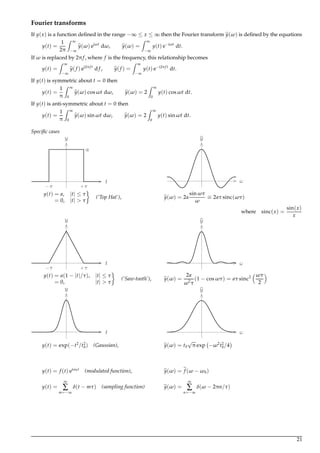
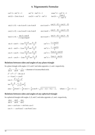
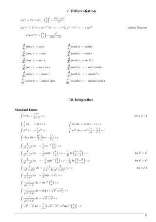
25. 15. Laplace Transforms
If y(t) is a function defined for t ≥ 0, the Laplace transform y(s) is defined by the equation
y(s) = L{y(t)} =
Z ∞
0
e−st
y(t) dt
Function y(t) (t > 0) Transform y(s)
δ(t) 1 Delta function
θ(t)
1
s
Unit step function
tn n!
sn+1
t
1/2
1
2
π
s3
t−1/2
π
s
e−at 1
(s + a)
sinωt
ω
(s2 + ω2
cosωt
s
(s2 + ω2)
sinh ωt
ω
(s2 − ω2)
coshωt
s
(s2 − ω2)
e−at
y(t) y(s + a)
y(t − τ) θ(t − τ) e−sτ
y(s)
ty(t) −
dy
ds
dy
dt
sy(s) − y(0)
dn
y
dtn
sn
y(s) − sn−1
y(0) − sn−2 dy
dt 0
· · · −
dn−1
y
dtn−1
0
Z t
0
y(τ) dτ
y(s)
s
Z t
0
x(τ) y(t − τ) dτ
Z t
0
x(t − τ) y(τ) dτ



x(s) y(s) Convolution theorem
[Note that if y(t) = 0 for t < 0 then the Fourier transform of y(t) is y(ω) = y(iω).]
23

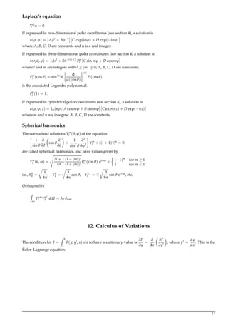
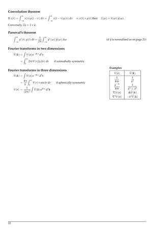
26. 16. Numerical Analysis
Finding the zeros of equations
If the equation is y = f (x) and xn is an approximation to the root then either
xn+1 = xn −
f (xn)
f (xn)
. (Newton)
or, xn+1 = xn −
xn − xn−1
f (xn) − f (xn−1)
f (xn) (Linear interpolation)
are, in general, better approximations.
Numerical integration of differential equations
If
dy
dx
= f (x, y) then
yn+1 = yn + h f (xn, yn) where h = xn+1 − xn (Euler method)
Putting y∗
n+1 = yn + h f (xn, yn) (improved Euler method)
then yn+1 = yn +
h[ f (xn, yn) + f (xn+1, y∗
n+1)]
2
Central difference notation
If y(x) is tabulated at equal intervals of x, where h is the interval, then δyn+1/2 = yn+1 − yn and
δ2
yn = δyn+1/2 − δyn−1/2
Approximating to derivatives
dy
dx n
≈
yn+1 − yn
h
≈
yn − yn−1
h
≈
δyn+1/2
+ δyn−1/2
2h
where h = xn+1 − xn
d2
y
dx2
n
≈
yn+1 − 2yn + yn−1
h2
=
δ2
yn
h2
Interpolation: Everett’s formula
y(x) = y(x0 + θh) ≈ θy0 + θy1 +
1
3!
θ(θ
2
− 1)δ2
y0 +
1
3!
θ(θ2
− 1)δ2
y1 + · · ·
where θ is the fraction of the interval h (= xn+1 − xn) between the sampling points and θ = 1 − θ. The first two
terms represent linear interpolation.
Numerical evaluation of definite integrals
Trapezoidal rule
The interval of integration is divided into n equal sub-intervals, each of width h; then
Z b
a
f (x) dx ≈ h c
1
2
f (a) + f (x1) + · · · + f (xj) + · · · +
1
2
f (b)
where h = (b − a)/n and xj = a + jh.
Simpson’s rule
The interval of integration is divided into an even number (say 2n) of equal sub-intervals, each of width h =
(b − a)/2n; then
Z b
a
f (x) dx ≈
h
3
f (a) + 4 f (x1) + 2 f (x2) + 4 f (x3) + · · · + 2 f (x2n−2) + 4 f (x2n−1) + f (b)
24

27. Gauss’s integration formulae
These have the general form
Z 1
−1
y(x) dx ≈
n
∑
1
ci y(xi)
For n = 2 : xi = ±0·5773; ci = 1, 1 (exact for any cubic).
For n = 3 : xi = −0·7746, 0·0, 0·7746; ci = 0·555, 0·888, 0·555 (exact for any quintic).
17. Treatment of Random Errors
Sample mean x =
1
n
(x1 + x2 + · · · xn)
Residual: d = x − x
Standard deviation of sample: s =
1
√
n
(d2
1 + d2
2 + · · · d2
n)1/2
Standard deviation of distribution: σ ≈
1
√
n − 1
(d2
1 + d2
2 + · · · d2
n)1/2
Standard deviation of mean: σm =
σ
√
n
=
1
n(n − 1)
(d2
1 + d2
2 + · · · d2
n)1/2
=
1
n(n − 1)
∑x2
i −
1
n ∑xi
2
1/2
Result of n measurements is quoted as x ± σm.
Range method
A quick but crude method of estimating σ is to find the range r of a set of n readings, i.e., the difference between
the largest and smallest values, then
σ ≈
r
√
n
.
This is usually adequate for n less than about 12.
Combination of errors
If Z = Z(A, B, . . .) (with A, B, etc. independent) then
(σZ)2
=
∂Z
∂A
σA
2
+
∂Z
∂B
σB
2
+ · · ·
So if
(i) Z = A ± B ± C, (σZ)2
= (σA)2
+ (σB)2
+ (σC)2
(ii) Z = AB or A/B,
σZ
Z
2
=
σA
A
2
+
σB
B
2
(iii) Z = Am
,
σZ
Z
= m
σA
A
(iv) Z = ln A, σZ =
σA
A
(v) Z = exp A,
σZ
Z
= σA
25

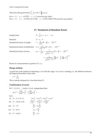
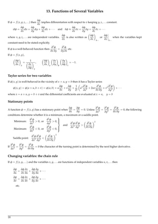
28. 18. Statistics
Mean and Variance
A random variable X has a distribution over some subset x of the real numbers. When the distribution of X is
discrete, the probability that X = xi is Pi. When the distribution is continuous, the probability that X lies in an
interval δx is f (x)δx, where f (x) is the probability density function.
Mean µ = E(X) = ∑Pixi or
Z
x f (x) dx.
Variance σ2
= V(X) = E[(X − µ)2
] = ∑Pi(xi − µ)2
or
Z
(x − µ)2
f (x) dx.
Probability distributions
Error function: erf(x) =
2
√
π
Z x
0
e−y2
dy
Binomial: f (x) =
n
x
px
qn−x
where q = (1 − p), µ = np, σ2
= npq, p < 1.
Poisson: f (x) =
µx
x!
e−µ
, and σ2
= µ
Normal: f (x) =
1
σ
√
2π
exp −
(x − µ)2
2σ2
Weighted sums of random variables
If W = aX + bY then E(W) = aE(X) + bE(Y). If X and Y are independent then V(W) = a2
V(X) + b2
V(Y).
Statistics of a data sample x1, . . . , xn
Sample mean x =
1
n ∑xi
Sample variance s2
=
1
n ∑(xi − x)2
=
1
n ∑x2
i − x2
= E(x2
) − [E(x)]2
Regression (least squares fitting)
To fit a straight line by least squares to n pairs of points (xi, yi), model the observations by yi = α + β(xi − x) + i,
where the i are independent samples of a random variable with zero mean and variance σ2
.
Sample statistics: s2
x =
1
n ∑(xi − x)2
, s2
y =
1
n ∑(yi − y)2
, s2
xy =
1
n ∑(xi − x)(yi − y).
Estimators: α = y, β =
s2
xy
s2
x
; E(Y at x) = α + β(x − x); σ2
=
n
n − 2
(residual variance),
where residual variance =
1
n ∑{yi − α − β(xi − x)}2
= s2
y −
s4
xy
s2
x
.
Estimates for the variances of α and β are
σ2
n
and
σ2
ns2
x
.
Correlation coefficient: ρ = r =
s2
xy
sxsy
.
26