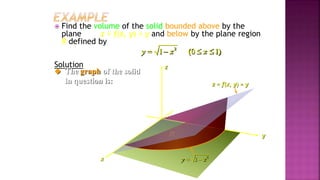
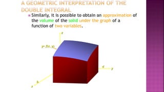
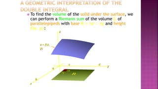
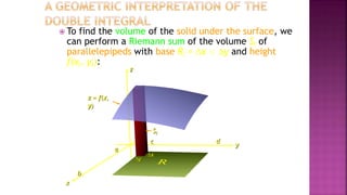
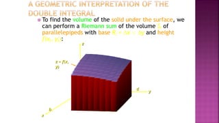
SlideShare a Scribd company logo
Double Integrals
z
x
y
2
1
y x
 
2
1
y x
 
R
z = f(x, y) = y
 You may recall that we can do a Riemann sum to
approximate the area under the graph of a function
of one variable by adding the areas of the
rectangles that form below the graph resulting from
small increments of x (x) within a given interval
[a, b]:
x
y
y= f(x)
a b
x
z
 Similarly, it is possible to obtain an approximation of
the volume of the solid under the graph of a
function of two variables.
y
x
a
b
c d
R
y= f(x, y)
a. Suppose g1(x) and g2(x) are continuous functions on [a, b] and
the region R is defined by R = {(x, y)| g1(x)  y  g2(x); a  x  b}.
Then,
2
1
( )
( )
( , ) ( , )
b g x
R a g x
f x y dA f x y dy dx
 

 
 
   
x
y
a b
y = g1(x)
y = g2(x)
R
 Let R be a region in the xy-plane and let f
be continuous and nonnegative on R.
 Then, the volume of the solid under a
surface bounded above by z = f(x, y) and
below by R is given by
( , )
R
V f x y dA
  
z
 To find the volume of the solid under the surface, we
can perform a Riemann sum of the volume Si of
parallelepipeds with base Ri = x ☓ y and height
f(xi, yi):
y
x
a
b
c d
x
y
z = f(x,
y)
R
z
 To find the volume of the solid under the surface, we
can perform a Riemann sum of the volume Si of
parallelepipeds with base Ri = x ☓ y and height
f(xi, yi):
y
x
a
b
c d
x
y
Si
z = f(x,
y)
R
y
a
b
c d
z
x
 To find the volume of the solid under the surface, we
can perform a Riemann sum of the volume Si of
parallelepipeds with base Ri = x ☓ y and height
f(xi, yi):
z = f(x,
y)
z
 The limit of the Riemann sum obtained when the number of
rectangles m along the x-axis, and the number of
subdivisions n along the y-axis tends to infinity is the value
of the double integral of f(x, y) over the region R and is
denoted by
z = f(x,
y)
y
x
a
b
c d
x
y
R
( , )
R
f x y dA
 
y ·n
x
·m
b. Suppose h1(y) and h2(y) are continuous functions on [c, d]
and the region R is defined by R = {(x, y)| h1(y)  x 
h2(y); c  y  d}.
Then, 2
1
( )
( )
( , ) ( , )
d h y
R c h y
f x y dA f x y dx dy
 

 
 
   
x
y
c
d
x = h1(y) x = h2(y)
R
4
3
2
1
1 2 3 4
 Evaluate ∫R∫f(x, y)dA given that f(x, y) = x2 + y2 and
R is the region bounded by the graphs of g1(x) = x
and g2(x) = 2x for 0  x  2.
Solution
 The region under consideration is:
x
g2(x) = 2x
R
y
g1(x) = x
Example 2, page 593
 Evaluate ∫R∫f(x, y)dA given that f(x, y) = x2 + y2 and
R is the region bounded by the graphs of g1(x) = x
and g2(x) = 2x for 0  x  2.
Solution
 Using Theorem 1, we find:
2 2
2 2
0
( , ) ( )
x
R x
f x y dA x y dy dx
 
 
 
 
   
2
2
2 3
0
1
3
x
x
x y y dx
 
 
 
 
 
 
 
 

2
3 3 3 3
0
8 1
2
3 3
x x x x dx
 
   
   
   
 
   
 

2
3
0
10
3
x dx
 
2
4
0
5
6
x
 1
3
13

Example 2, page 593
1
1
 Evaluate ∫R∫f(x, y)dA, where f(x, y) = xey and R is the
plane region bounded by the graphs of y = x2 and y = x.
Solution
 The region under consideration is:
x
g1(x) = x2
R
y
g2(x) = x
 The points of intersection of
the two curves are found by
solving the equation x2 = x,
giving x = 0 and x = 1.
Example 3, page 593
 Evaluate ∫R∫f(x, y)dA, where f(x, y) = xey and R is
the plane region bounded by the graphs of y = x2
and y = x.
Solution
 Using Theorem 1, we find:
2
1
0
( , )
x
y
R x
f x y dA xe dy dx
 

 
 
      2
1
0
x
y
x
xe dx
 

 
 

2
1
0
( )
x x
xe xe dx
 

2
1 1
0 0
x x
xe dx xe dx
 
 
2
1
0
1
( 1)
2
x x
x e e
 
  
 
 
1 1 1
1 (3 )
2 2 2
e e
 
      
 
 
Integrating by parts on
the right-hand side
Example 3, page 593
 Find the volume of the solid bounded above by the
plane z = f(x, y) = y and below by the plane
region R defined by
Solution
 The graph of the region R is:
1
1
x
y
2
1
y x
 
R
 Observe that f(x, y) = y > 0 for (x, y) ∈ R.
2
1 (0 1)
y x x
   
Example 4, page 594
 Find the volume of the solid bounded above by the
plane z = f(x, y) = y and below by the plane
region R defined by
Solution
 Therefore, the required volume is given by
2
1 1
0 0
x
R
V ydA ydy dx

 
   
 
   
2
1
1
2
0
0
1
2
x
y dx

 
 

 
 

1
2
0
1
(1 )
2
x dx
 

1
3
0
1 1
2 3
x x
 
 
 
 
1
3

2
1 (0 1)
y x x
   
Example 4, page 594
 Find the volume of the solid bounded above by the
plane z = f(x, y) = y and below by the plane region
R defined by
Solution
2
1 (0 1)
y x x
   
z
x
y
 The graph of the solid
in question is:
2
1
y x
 
R
z = f(x, y) = y
Example 4, page 594

More Related Content

Similar to double integral.pptx

Calculusseveralvariables.ppt
Calculusseveralvariables.pptCalculusseveralvariables.ppt
Calculusseveralvariables.ppt
ssuser055963
 
Double_Integral.pdf
Double_Integral.pdfDouble_Integral.pdf
Double_Integral.pdf
d00a7ece
 
5.4 more areas
5.4 more areas5.4 more areas
5.4 more areasmath265
 
Relations & functions.pps
Relations  &  functions.ppsRelations  &  functions.pps
Relations & functions.ppsindu psthakur
 
24 double integral over polar coordinate
24 double integral over polar coordinate24 double integral over polar coordinate
24 double integral over polar coordinatemath267
 
Lesson 16 length of an arc
Lesson 16 length of an arcLesson 16 length of an arc
Lesson 16 length of an arc
Lawrence De Vera
 
Introduccio al calculo vectorial
Introduccio  al calculo vectorialIntroduccio  al calculo vectorial
Introduccio al calculo vectorial
EDESMITCRUZ1
 
Tcu12 crc multi
Tcu12 crc multiTcu12 crc multi
Tcu12 crc multi
Sahiris Seg
 
1523 double integrals
1523 double integrals1523 double integrals
1523 double integrals
Dr Fereidoun Dejahang
 
exponential functions and their graphs.ppt
exponential functions and their graphs.pptexponential functions and their graphs.ppt
exponential functions and their graphs.ppt
TonetSalagoCantere
 
Chatper 15
Chatper 15Chatper 15
Chatper 15
EasyStudy3
 
Chapter3partialderivatives 150105021210-conversion-gate02
Chapter3partialderivatives 150105021210-conversion-gate02Chapter3partialderivatives 150105021210-conversion-gate02
Chapter3partialderivatives 150105021210-conversion-gate02
Cleophas Rwemera
 
Applied Calculus Chapter 3 partial derivatives
Applied Calculus Chapter  3 partial derivativesApplied Calculus Chapter  3 partial derivatives
Applied Calculus Chapter 3 partial derivatives
J C
 
3. Quadrature Complete Theory Module-5.pdf
3. Quadrature Complete Theory Module-5.pdf3. Quadrature Complete Theory Module-5.pdf
3. Quadrature Complete Theory Module-5.pdf
RajuSingh806014
 
Lesson 11 plane areas area by integration
Lesson 11 plane areas area by integrationLesson 11 plane areas area by integration
Lesson 11 plane areas area by integration
Lawrence De Vera
 
22 double integrals
22 double integrals22 double integrals
22 double integralsmath267
 
Superficies regulares planos tangentes y normales
Superficies regulares  planos tangentes y  normales Superficies regulares  planos tangentes y  normales
Superficies regulares planos tangentes y normales
EDESMITCRUZ1
 
Differential calculus
Differential calculus  Differential calculus
Differential calculus
Santhanam Krishnan
 
Mathematics 3.pdf civil engineering concrete
Mathematics 3.pdf civil engineering concreteMathematics 3.pdf civil engineering concrete
Mathematics 3.pdf civil engineering concrete
mocr84810
 

Similar to double integral.pptx (20)

Calculusseveralvariables.ppt
Calculusseveralvariables.pptCalculusseveralvariables.ppt
Calculusseveralvariables.ppt
 
Double_Integral.pdf
Double_Integral.pdfDouble_Integral.pdf
Double_Integral.pdf
 
Directional derivative and gradient
Directional derivative and gradientDirectional derivative and gradient
Directional derivative and gradient
 
5.4 more areas
5.4 more areas5.4 more areas
5.4 more areas
 
Relations & functions.pps
Relations  &  functions.ppsRelations  &  functions.pps
Relations & functions.pps
 
24 double integral over polar coordinate
24 double integral over polar coordinate24 double integral over polar coordinate
24 double integral over polar coordinate
 
Lesson 16 length of an arc
Lesson 16 length of an arcLesson 16 length of an arc
Lesson 16 length of an arc
 
Introduccio al calculo vectorial
Introduccio  al calculo vectorialIntroduccio  al calculo vectorial
Introduccio al calculo vectorial
 
Tcu12 crc multi
Tcu12 crc multiTcu12 crc multi
Tcu12 crc multi
 
1523 double integrals
1523 double integrals1523 double integrals
1523 double integrals
 
exponential functions and their graphs.ppt
exponential functions and their graphs.pptexponential functions and their graphs.ppt
exponential functions and their graphs.ppt
 
Chatper 15
Chatper 15Chatper 15
Chatper 15
 
Chapter3partialderivatives 150105021210-conversion-gate02
Chapter3partialderivatives 150105021210-conversion-gate02Chapter3partialderivatives 150105021210-conversion-gate02
Chapter3partialderivatives 150105021210-conversion-gate02
 
Applied Calculus Chapter 3 partial derivatives
Applied Calculus Chapter  3 partial derivativesApplied Calculus Chapter  3 partial derivatives
Applied Calculus Chapter 3 partial derivatives
 
3. Quadrature Complete Theory Module-5.pdf
3. Quadrature Complete Theory Module-5.pdf3. Quadrature Complete Theory Module-5.pdf
3. Quadrature Complete Theory Module-5.pdf
 
Lesson 11 plane areas area by integration
Lesson 11 plane areas area by integrationLesson 11 plane areas area by integration
Lesson 11 plane areas area by integration
 
22 double integrals
22 double integrals22 double integrals
22 double integrals
 
Superficies regulares planos tangentes y normales
Superficies regulares  planos tangentes y  normales Superficies regulares  planos tangentes y  normales
Superficies regulares planos tangentes y normales
 
Differential calculus
Differential calculus  Differential calculus
Differential calculus
 
Mathematics 3.pdf civil engineering concrete
Mathematics 3.pdf civil engineering concreteMathematics 3.pdf civil engineering concrete
Mathematics 3.pdf civil engineering concrete
 

Recently uploaded

HYDROPOWER - Hydroelectric power generation
HYDROPOWER - Hydroelectric power generationHYDROPOWER - Hydroelectric power generation
HYDROPOWER - Hydroelectric power generation
Robbie Edward Sayers
 
power quality voltage fluctuation UNIT - I.pptx
power quality voltage fluctuation UNIT - I.pptxpower quality voltage fluctuation UNIT - I.pptx
power quality voltage fluctuation UNIT - I.pptx
ViniHema
 
Nuclear Power Economics and Structuring 2024
Nuclear Power Economics and Structuring 2024Nuclear Power Economics and Structuring 2024
Nuclear Power Economics and Structuring 2024
Massimo Talia
 
Automobile Management System Project Report.pdf
Automobile Management System Project Report.pdfAutomobile Management System Project Report.pdf
Automobile Management System Project Report.pdf
Kamal Acharya
 
Event Management System Vb Net Project Report.pdf
Event Management System Vb Net  Project Report.pdfEvent Management System Vb Net  Project Report.pdf
Event Management System Vb Net Project Report.pdf
Kamal Acharya
 
在线办理(ANU毕业证书)澳洲国立大学毕业证录取通知书一模一样
在线办理(ANU毕业证书)澳洲国立大学毕业证录取通知书一模一样在线办理(ANU毕业证书)澳洲国立大学毕业证录取通知书一模一样
在线办理(ANU毕业证书)澳洲国立大学毕业证录取通知书一模一样
obonagu
 
Quality defects in TMT Bars, Possible causes and Potential Solutions.
Quality defects in TMT Bars, Possible causes and Potential Solutions.Quality defects in TMT Bars, Possible causes and Potential Solutions.
Quality defects in TMT Bars, Possible causes and Potential Solutions.
PrashantGoswami42
 
Design and Analysis of Algorithms-DP,Backtracking,Graphs,B&B
Design and Analysis of Algorithms-DP,Backtracking,Graphs,B&BDesign and Analysis of Algorithms-DP,Backtracking,Graphs,B&B
Design and Analysis of Algorithms-DP,Backtracking,Graphs,B&B
Sreedhar Chowdam
 
Gen AI Study Jams _ For the GDSC Leads in India.pdf
Gen AI Study Jams _ For the GDSC Leads in India.pdfGen AI Study Jams _ For the GDSC Leads in India.pdf
Gen AI Study Jams _ For the GDSC Leads in India.pdf
gdsczhcet
 
Planning Of Procurement o different goods and services
Planning Of Procurement o different goods and servicesPlanning Of Procurement o different goods and services
Planning Of Procurement o different goods and services
JoytuBarua2
 
H.Seo, ICLR 2024, MLILAB, KAIST AI.pdf
H.Seo,  ICLR 2024, MLILAB,  KAIST AI.pdfH.Seo,  ICLR 2024, MLILAB,  KAIST AI.pdf
H.Seo, ICLR 2024, MLILAB, KAIST AI.pdf
MLILAB
 
Courier management system project report.pdf
Courier management system project report.pdfCourier management system project report.pdf
Courier management system project report.pdf
Kamal Acharya
 
Water Industry Process Automation and Control Monthly - May 2024.pdf
Water Industry Process Automation and Control Monthly - May 2024.pdfWater Industry Process Automation and Control Monthly - May 2024.pdf
Water Industry Process Automation and Control Monthly - May 2024.pdf
Water Industry Process Automation & Control
 
WATER CRISIS and its solutions-pptx 1234
WATER CRISIS and its solutions-pptx 1234WATER CRISIS and its solutions-pptx 1234
WATER CRISIS and its solutions-pptx 1234
AafreenAbuthahir2
 
ethical hacking-mobile hacking methods.ppt
ethical hacking-mobile hacking methods.pptethical hacking-mobile hacking methods.ppt
ethical hacking-mobile hacking methods.ppt
Jayaprasanna4
 
Democratizing Fuzzing at Scale by Abhishek Arya
Democratizing Fuzzing at Scale by Abhishek AryaDemocratizing Fuzzing at Scale by Abhishek Arya
Democratizing Fuzzing at Scale by Abhishek Arya
abh.arya
 
TECHNICAL TRAINING MANUAL GENERAL FAMILIARIZATION COURSE
TECHNICAL TRAINING MANUAL   GENERAL FAMILIARIZATION COURSETECHNICAL TRAINING MANUAL   GENERAL FAMILIARIZATION COURSE
TECHNICAL TRAINING MANUAL GENERAL FAMILIARIZATION COURSE
DuvanRamosGarzon1
 
ethical hacking in wireless-hacking1.ppt
ethical hacking in wireless-hacking1.pptethical hacking in wireless-hacking1.ppt
ethical hacking in wireless-hacking1.ppt
Jayaprasanna4
 
DESIGN A COTTON SEED SEPARATION MACHINE.docx
DESIGN A COTTON SEED SEPARATION MACHINE.docxDESIGN A COTTON SEED SEPARATION MACHINE.docx
DESIGN A COTTON SEED SEPARATION MACHINE.docx
FluxPrime1
 
CME397 Surface Engineering- Professional Elective
CME397 Surface Engineering- Professional ElectiveCME397 Surface Engineering- Professional Elective
CME397 Surface Engineering- Professional Elective
karthi keyan
 

Recently uploaded (20)

HYDROPOWER - Hydroelectric power generation
HYDROPOWER - Hydroelectric power generationHYDROPOWER - Hydroelectric power generation
HYDROPOWER - Hydroelectric power generation
 
power quality voltage fluctuation UNIT - I.pptx
power quality voltage fluctuation UNIT - I.pptxpower quality voltage fluctuation UNIT - I.pptx
power quality voltage fluctuation UNIT - I.pptx
 
Nuclear Power Economics and Structuring 2024
Nuclear Power Economics and Structuring 2024Nuclear Power Economics and Structuring 2024
Nuclear Power Economics and Structuring 2024
 
Automobile Management System Project Report.pdf
Automobile Management System Project Report.pdfAutomobile Management System Project Report.pdf
Automobile Management System Project Report.pdf
 
Event Management System Vb Net Project Report.pdf
Event Management System Vb Net  Project Report.pdfEvent Management System Vb Net  Project Report.pdf
Event Management System Vb Net Project Report.pdf
 
在线办理(ANU毕业证书)澳洲国立大学毕业证录取通知书一模一样
在线办理(ANU毕业证书)澳洲国立大学毕业证录取通知书一模一样在线办理(ANU毕业证书)澳洲国立大学毕业证录取通知书一模一样
在线办理(ANU毕业证书)澳洲国立大学毕业证录取通知书一模一样
 
Quality defects in TMT Bars, Possible causes and Potential Solutions.
Quality defects in TMT Bars, Possible causes and Potential Solutions.Quality defects in TMT Bars, Possible causes and Potential Solutions.
Quality defects in TMT Bars, Possible causes and Potential Solutions.
 
Design and Analysis of Algorithms-DP,Backtracking,Graphs,B&B
Design and Analysis of Algorithms-DP,Backtracking,Graphs,B&BDesign and Analysis of Algorithms-DP,Backtracking,Graphs,B&B
Design and Analysis of Algorithms-DP,Backtracking,Graphs,B&B
 
Gen AI Study Jams _ For the GDSC Leads in India.pdf
Gen AI Study Jams _ For the GDSC Leads in India.pdfGen AI Study Jams _ For the GDSC Leads in India.pdf
Gen AI Study Jams _ For the GDSC Leads in India.pdf
 
Planning Of Procurement o different goods and services
Planning Of Procurement o different goods and servicesPlanning Of Procurement o different goods and services
Planning Of Procurement o different goods and services
 
H.Seo, ICLR 2024, MLILAB, KAIST AI.pdf
H.Seo,  ICLR 2024, MLILAB,  KAIST AI.pdfH.Seo,  ICLR 2024, MLILAB,  KAIST AI.pdf
H.Seo, ICLR 2024, MLILAB, KAIST AI.pdf
 
Courier management system project report.pdf
Courier management system project report.pdfCourier management system project report.pdf
Courier management system project report.pdf
 
Water Industry Process Automation and Control Monthly - May 2024.pdf
Water Industry Process Automation and Control Monthly - May 2024.pdfWater Industry Process Automation and Control Monthly - May 2024.pdf
Water Industry Process Automation and Control Monthly - May 2024.pdf
 
WATER CRISIS and its solutions-pptx 1234
WATER CRISIS and its solutions-pptx 1234WATER CRISIS and its solutions-pptx 1234
WATER CRISIS and its solutions-pptx 1234
 
ethical hacking-mobile hacking methods.ppt
ethical hacking-mobile hacking methods.pptethical hacking-mobile hacking methods.ppt
ethical hacking-mobile hacking methods.ppt
 
Democratizing Fuzzing at Scale by Abhishek Arya
Democratizing Fuzzing at Scale by Abhishek AryaDemocratizing Fuzzing at Scale by Abhishek Arya
Democratizing Fuzzing at Scale by Abhishek Arya
 
TECHNICAL TRAINING MANUAL GENERAL FAMILIARIZATION COURSE
TECHNICAL TRAINING MANUAL   GENERAL FAMILIARIZATION COURSETECHNICAL TRAINING MANUAL   GENERAL FAMILIARIZATION COURSE
TECHNICAL TRAINING MANUAL GENERAL FAMILIARIZATION COURSE
 
ethical hacking in wireless-hacking1.ppt
ethical hacking in wireless-hacking1.pptethical hacking in wireless-hacking1.ppt
ethical hacking in wireless-hacking1.ppt
 
DESIGN A COTTON SEED SEPARATION MACHINE.docx
DESIGN A COTTON SEED SEPARATION MACHINE.docxDESIGN A COTTON SEED SEPARATION MACHINE.docx
DESIGN A COTTON SEED SEPARATION MACHINE.docx
 
CME397 Surface Engineering- Professional Elective
CME397 Surface Engineering- Professional ElectiveCME397 Surface Engineering- Professional Elective
CME397 Surface Engineering- Professional Elective
 

double integral.pptx

  • 1. Double Integrals z x y 2 1 y x   2 1 y x   R z = f(x, y) = y
  • 2.  You may recall that we can do a Riemann sum to approximate the area under the graph of a function of one variable by adding the areas of the rectangles that form below the graph resulting from small increments of x (x) within a given interval [a, b]: x y y= f(x) a b x
  • 3. z  Similarly, it is possible to obtain an approximation of the volume of the solid under the graph of a function of two variables. y x a b c d R y= f(x, y)
  • 4. a. Suppose g1(x) and g2(x) are continuous functions on [a, b] and the region R is defined by R = {(x, y)| g1(x)  y  g2(x); a  x  b}. Then, 2 1 ( ) ( ) ( , ) ( , ) b g x R a g x f x y dA f x y dy dx            x y a b y = g1(x) y = g2(x) R
  • 5.  Let R be a region in the xy-plane and let f be continuous and nonnegative on R.  Then, the volume of the solid under a surface bounded above by z = f(x, y) and below by R is given by ( , ) R V f x y dA   
  • 6. z  To find the volume of the solid under the surface, we can perform a Riemann sum of the volume Si of parallelepipeds with base Ri = x ☓ y and height f(xi, yi): y x a b c d x y z = f(x, y) R
  • 7. z  To find the volume of the solid under the surface, we can perform a Riemann sum of the volume Si of parallelepipeds with base Ri = x ☓ y and height f(xi, yi): y x a b c d x y Si z = f(x, y) R
  • 8. y a b c d z x  To find the volume of the solid under the surface, we can perform a Riemann sum of the volume Si of parallelepipeds with base Ri = x ☓ y and height f(xi, yi): z = f(x, y)
  • 9. z  The limit of the Riemann sum obtained when the number of rectangles m along the x-axis, and the number of subdivisions n along the y-axis tends to infinity is the value of the double integral of f(x, y) over the region R and is denoted by z = f(x, y) y x a b c d x y R ( , ) R f x y dA   y ·n x ·m
  • 10. b. Suppose h1(y) and h2(y) are continuous functions on [c, d] and the region R is defined by R = {(x, y)| h1(y)  x  h2(y); c  y  d}. Then, 2 1 ( ) ( ) ( , ) ( , ) d h y R c h y f x y dA f x y dx dy            x y c d x = h1(y) x = h2(y) R
  • 11. 4 3 2 1 1 2 3 4  Evaluate ∫R∫f(x, y)dA given that f(x, y) = x2 + y2 and R is the region bounded by the graphs of g1(x) = x and g2(x) = 2x for 0  x  2. Solution  The region under consideration is: x g2(x) = 2x R y g1(x) = x Example 2, page 593
  • 12.  Evaluate ∫R∫f(x, y)dA given that f(x, y) = x2 + y2 and R is the region bounded by the graphs of g1(x) = x and g2(x) = 2x for 0  x  2. Solution  Using Theorem 1, we find: 2 2 2 2 0 ( , ) ( ) x R x f x y dA x y dy dx             2 2 2 3 0 1 3 x x x y y dx                  2 3 3 3 3 0 8 1 2 3 3 x x x x dx                        2 3 0 10 3 x dx   2 4 0 5 6 x  1 3 13  Example 2, page 593
  • 13. 1 1  Evaluate ∫R∫f(x, y)dA, where f(x, y) = xey and R is the plane region bounded by the graphs of y = x2 and y = x. Solution  The region under consideration is: x g1(x) = x2 R y g2(x) = x  The points of intersection of the two curves are found by solving the equation x2 = x, giving x = 0 and x = 1. Example 3, page 593
  • 14.  Evaluate ∫R∫f(x, y)dA, where f(x, y) = xey and R is the plane region bounded by the graphs of y = x2 and y = x. Solution  Using Theorem 1, we find: 2 1 0 ( , ) x y R x f x y dA xe dy dx              2 1 0 x y x xe dx         2 1 0 ( ) x x xe xe dx    2 1 1 0 0 x x xe dx xe dx     2 1 0 1 ( 1) 2 x x x e e          1 1 1 1 (3 ) 2 2 2 e e              Integrating by parts on the right-hand side Example 3, page 593
  • 15.  Find the volume of the solid bounded above by the plane z = f(x, y) = y and below by the plane region R defined by Solution  The graph of the region R is: 1 1 x y 2 1 y x   R  Observe that f(x, y) = y > 0 for (x, y) ∈ R. 2 1 (0 1) y x x     Example 4, page 594
  • 16.  Find the volume of the solid bounded above by the plane z = f(x, y) = y and below by the plane region R defined by Solution  Therefore, the required volume is given by 2 1 1 0 0 x R V ydA ydy dx              2 1 1 2 0 0 1 2 x y dx            1 2 0 1 (1 ) 2 x dx    1 3 0 1 1 2 3 x x         1 3  2 1 (0 1) y x x     Example 4, page 594
  • 17.  Find the volume of the solid bounded above by the plane z = f(x, y) = y and below by the plane region R defined by Solution 2 1 (0 1) y x x     z x y  The graph of the solid in question is: 2 1 y x   R z = f(x, y) = y Example 4, page 594