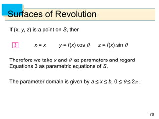
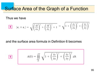
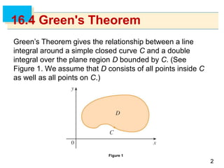
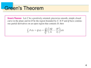
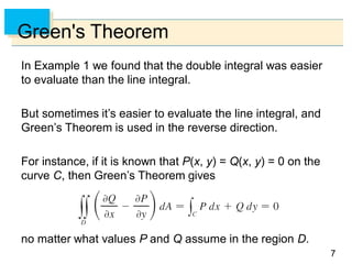
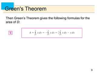
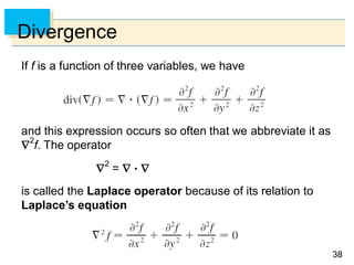
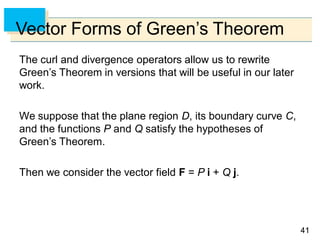
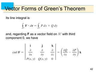
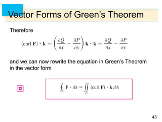
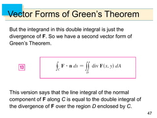
- Green's Theorem relates a line integral around a closed curve C to a double integral over the region D bounded by C. It expresses the line integral as the double integral of the curl or divergence of the vector field over D.
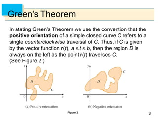
- The curl and divergence operators can be used to write Green's Theorem in vector forms involving the tangential and normal components of the vector field along C.
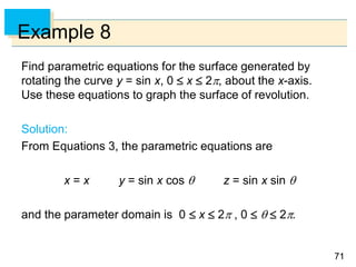
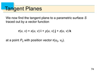
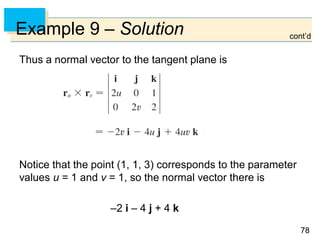
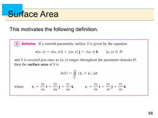
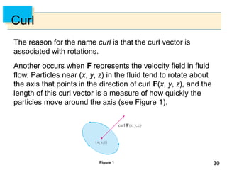
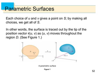
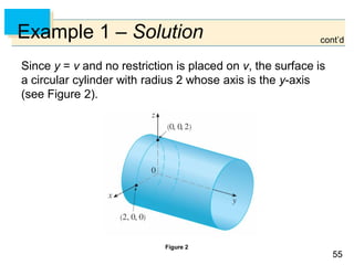
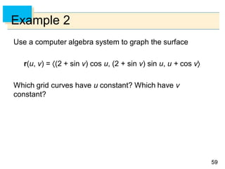
- Parametric surfaces in 3D space can be described by a vector-valued function r(u,v) of two parameters u and v. The set of points traced out by this function as u and v vary is the parametric surface.


![6565
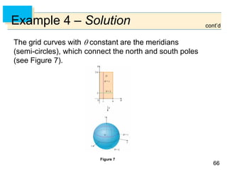
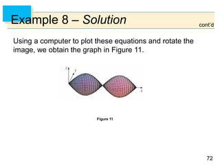
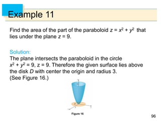
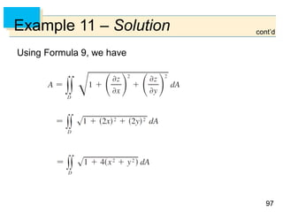
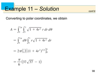
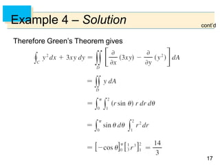
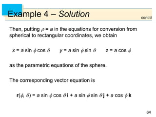
Example 4 – Solution
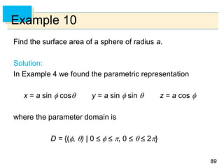
We have 0 and 0 2, so the parameter
domain is the rectangle D = [0, ] [0, 2].
The grid curves with constant are the circles of constant
latitude (including the equator).
cont’d](https://image.slidesharecdn.com/chapter16-2-191022223141/85/Chapter-16-2-65-320.jpg)