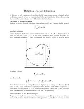
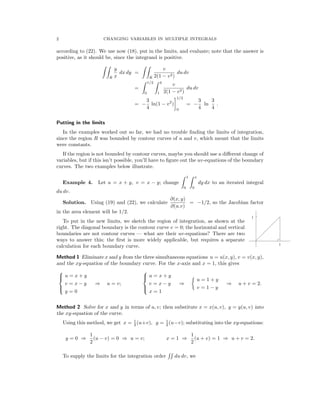
Here are the steps to solve this problem: 1. The region R is bounded by the circle r = 1 and the line x + y = 1 in polar coordinates. 2. To set up the double integral in polar coordinates, we first identify the limits of integration with respect to r. Since we are integrating r dr first, we hold θ fixed and let r vary from the minimum to maximum r value along each radial line. The minimum is r = 1/(cosθ + sinθ) and the maximum is r = 1. 3. Next, we identify the limits with respect to θ. The radial lines intersecting the region range from θ = 0 to θ = π/2. 4.

1. � �
�
�
Definition of double integration
In this note we will work abstractly, defining double integration as a sum, technically a limit
of Riemann sums. It is best to learn this first before getting into the details of computing
the value of a double integral –we will learn how to do that next.
Definition of double integrals
Suppose we have a region in the plane R and a function f(x, y), Then the double integral
f(x, y) dA
R
is defined as follows.
Divide the region R into small pieces, numbered from 1 to n. Let ΔAi be the area of the ith
piece and also pick a point (xi, yi) in that piece. The figure shows a region R divided into
small pieces and shows the ith piece with its area, and choice of a point in the little region.
y
x
R
• (xi, yi)
area = ΔAi
Now form the sum
n
f(xi, yi) ΔAi,
i=1
and then, finally
� � n
f(x, y) dA = lim f(xi, yi) ΔAi.
R ΔA 0
→
i=1
Here, the limit is taken by letting the number of pieces go to infinity and the area of each
piece go to 0. There are technical requirements that the limit exist and be independent of
the specific limiting process. In 18.02 these requirements are always met. (Later you might
study fractals and other strange objects which don’t satisfy them.)
Interpretations of the double integral
As you saw in single variable calculus, these sums can be used to compute areas, volumes,
mass, work, moment of inertia and many other quantities. Again, before focusung on some

2. � �
� �
computational issues we will show you how easy it is to setup a double integral to compute
certain quantities.
Example 1: Set up a double integral to compute the area of a region R in the plane.
Answer: Use the figure above for visualization. The area of R is just the sum of the areas
of the pieces. That is, � �
area = dA.
R
Example 2: Set up a double integral to compute the volume of the solid below the graph
of z = f(x, y) = 2 − .5(x + y) and above the unit square in the xy-plane.
Answer: The figure below shows the graph of f(x, y) above the unit square in the plane.
The unit square is labeled R. We also show a little piece of the R and the solid region above
that piece. We are imagining we’ve divided R into n small pieces and this is the ith one. It
contains the point (xi, yi) and has area ΔAi.
z
y
1
1
R
• (xi, yi), area = ΔAi
x
The small solid region is almost a box and so its volume, ΔVi, is roughly its base times its
height, i.e.,
ΔVi ≈ ΔAi × f(xi, yi).
The total volume is the sum of the volumes of all the small pieces, i.e.,
n n
volume = ΔVi ≈ ΔAi × f(xi, yi).
i=1 i=1
In the limit this becomes an exact integral for volume
volume = f(x, y) dA.
R

8. Limits in Iterated Integrals
For most students, the trickiest part of evaluating multiple integrals by iteration is to
put in the limits of integration. Fortunately, a fairly uniform procedure is available which
works in any coordinate system. You must always begin by sketching the region; in what
follows we’ll assume you’ve done this.
x+y=1
2 2
x +y =1
1. Double integrals in rectangular coordinates.
Let’s illustrate this procedure on the first case that’s usually
taken up: double integrals in rectangular coordinates. Suppose we
want to evaluate over the region R pictured the integral
� �
f(x, y) dy dx , R = region between x2
+ y2
= 1 and x + y = 1 ;
R
we are integrating first with respect to y. Then to put in the limits,
1. Hold x fixed, and let y increase (since we are integrating with respect to y).
As the point (x, y) moves, it traces out a vertical line.
2. Integrate from the y-value where this vertical line enters the region R, to
the y-value where it leaves R.
3. Then let x increase, integrating from the lowest x-value for which the vertical
line intersects R, to the highest such x-value.
Carrying out this program for the region R pictured, the vertical line enters R where
√
y = 1 − x, and leaves where y = 1 − x2.
y= -x
y=
1
1-x2
The vertical lines which intersect R are those between x = 0 and
x = 1. Thus we get for the limits:
� � � � √
1 1−x2
f(x, y) dy dx = f(x, y) dy dx.
R 0 1−x
To calculate the double integral, integrating in the reverse order
��
R
f(x, y) dx dy,
1. Hold y fixed, let x increase (since we are integrating first with respect to x).
This traces out a horizontal line.
2. Integrate from the x-value where the horizontal line enters R to the x-value
where it leaves.
3. Choose the y-limits to include all of the horizontal lines which intersect R
x= -y
1
.
x=1-y2
Following this prescription with our integral we get:
� � � � √
1 1−y2
f(x, y) dx dy = f(x, y) dx dy.
R 0 1−y
1

16. 1
1
Tetrahedron
��
Problems: Regions of Integration
1. Find the mass of the region R bounded by
y = x + 1; y = x2; x = 0 and x = 1, if density = δ(x, y) = xy.
2. Find the volume of the tetrahedron shown below.
z = f(x, y)
1

17. y = x + 1
R
y = x2
1
��
Problems: Regions of Integration
1. Find the mass of the region R bounded by
y = x + 1; y = x2; x = 0 and x = 1, if density = δ(x, y) = xy.
Answer:
Inner limits: 2
⇒
M =
y from x to x + 1.
1
Outer limits: x from 0 to 1.
x+1
dA
δ(x, y) = xy dy dx
R x=0 y=x2
x+1 2
[x+1 2
y 5 3
x(x + 1) x x x x5
Inner: xy dy =
x
=
−
=
+ 2
x +
x
−
.
x2 2
2 2 2 2 2 2
1 3 5 4 3 2 6 1
x
2 x
[
[
[
x
x x
x
x
[
1 1 1 1 5
Outer:
+ x
+
− dx = + +
= + +
= .
0 2 2 2 8 3 4
−
12
0 8 3 4
−
12 8
Note: The syntax y = x2 in limits is redundant but useful.
[
[
We know it must be y because
of the dy matching the integral sign.
[
2. Find the volume of the tetrahedron shown below.
1 z = f(x, y)
1
1
Tetrahedron
Answer: The surface has height: z = 1 − x − y.
y
1
y = 1 − x
R
x
1
Region R
1 1−x
Limits: inner: 0 < y < 1 − x, outer: 0 < x < 1. ⇒ V = 1 x y dy dx.
[
x=0 y=0
−
−
1−x 1
y2 −x
1 x2
Inner:
1 − x − y dy = y − xy −
[
[
[
2
= 1 − x − x + x − + x − .
y=0 2 0 2 2
1
1 x2 1 1 1 1
Outer: − x + dx = − + = .
0 2 2 2 2 6 6
1

18. �
�
�
�
�
Changing the order of integration
1. Evaluate � π/2 � π/2
sin y
I = dy dx
0 x y
by changing the order of integration.
Answer:
The given limits are (inner) y from x to π/2; (outer) x from 0 to π/2.
We use these to sketch the region of integration.
y
The given limits have inner variable y. To reverse the order of integration we use horizontal
stripes. The limits in this order are
(inner) x from 0 to y; (outer) y from 0 to π/2.
x
y = x
π/2
π/2
So the integral becomes
� π/2 y
sin y
I
=
dx dy
0 0 y
We compute the inner, then the outer integrals.
y
sin y
π/2
Inner:
= sin y. Outer:
= 1.
x
− cos y|
0
y
0

22. Problems: Exchanging the Order of Integration
� 2 � 2
−y2
Calculate e dy dx.
0 x

23. Problems: Exchanging the Order of Integration
2 2
−y2
Calculate e dy dx.
0 x
Answer: As you
2
may recall, the function e−y has no simple antiderivative. However, this
double integral can be computed by reversing the order of integration.
The region R is the triangle with vertices at (0, 0), (0, 2) and (2, 2) (sketch it!) Thus:
2 2 2
y
−y2
dx
2
e dy =
=0
−y
.
x
e dx dy
y=x y=0 x=0
y
− 2
Inner:
e
y
dx = ye
− 2
y
.
x=0
2 2
2
Outer: −y2 1
1 1
ye dy = − e
−y 4
=
(1 e
−
) .
y=0 2
0 2
− ≈
2
We’re finding the area under a surface with maximum height 1 and minimum height e−4 ≈
0.1 over a triangle of area 2. This answer seems plausible.

24. �
Integration in polar coordinates
Polar Coordinates
Polar coordinates are a different way of describing points in the plane. The polar coordinates
(r, θ) are related to the usual rectangular coordinates (x, y) by by
x = r cos θ, y = r sin θ
The figure below shows the standard polar triangle relating x, y, r and θ.
y
x
��
��
x
y
r
θ
Because cos and sin are periodic, different (r, θ) can represent the same point in the plane.
The table below shows this for a few points.
(x, y) (1, 0) (0, 1) (2, 0) (1, 1) (−1, 1) (−1, −1) (0, 0)
(r, θ) (1, 0) (1, π/2) (2, 0) (
√
2, π/4) (
√
2, 3π/4) (
√
2, 5π/4) (0, π/2)
(r, θ) (1, 2π) (
√
2, 9π/4) (−
√
2, π/4) (0, −7.2)
(r, θ) (1, 4π)
In fact, you can add any multiple of 2π to θ and the polar coordinates will still represent
the same point.
Because θ is not uniquely specified it’s a little trickier going from rectangular to polar
coordinates. The equations are easily deduced from the standard polar triangle.
2
r = x2 + y , ”θ = tan−1
(y/x)”.
We use quotes around tan−1 to indicate it is not a single valued function.
The area element in polar coordinates
In polar coordinates the area element is given by
dA = r dr dθ.
The geometric justification for this is shown in by the following figure.
x
��
y
��
•
Δθ r
r
Δr
rΔθ
ΔA
The small curvy rectangle has sides Δr and rΔθ, thus its area satisfies ΔA ≈ (Δr)(r Δθ).
As usual, in the limit this becomes dA = r dr dθ.

25. � �
�
�
Double integrals in polar coordinates
The area element is one piece of a double integral, the other piece is the limits of integration
which describe the region being integrated over.
Finding procedure for finding the limits in polar coordinates is the same as for rectangular
coordinates. Suppose we want to evaluate dr dθ over the region R shown.
R
x
��
y
��
x + y = 1
x
��
y
��
R
��
•r = 1
(The integrand, including the r that usually goes with r dr dθ, is irrelevant here, and there­
fore omitted.)
As usual, we integrate first with respect to r. Therefore, we
1. Hold θ fixed, and let r increase (since we are integrating with respect to r). As the point
moves, it traces out a ray going out from the origin.
2. Integrate from the r-value where the ray enters R to the r-value where it leaves. This
gives the limits on r.
3. Integrate from the lowest value of θ for which the corresponding ray intersects R to the
highest value of θ.
To follow this procedure, we need the equation of the line in polar coordinates. We have
x + y = 1 → r cos θ + r sin θ = 1, or r =
1
cos θ + sin θ
.
This is the r value where the ray enters the region; it leaves where r = 1. The rays which
intersect R lie between θ = 0 and θ = π/2. Thus the double iterated integral in polar
coordinates has the limits � π/2
0
� 1
1/(cos θ+sin θ)
dr dθ.
Example: Find the mass of the region R shown if it has density δ(x, y) = xy (in units of
mass/unit area)
In polar coordinates: δ = r2 cos θ sin θ.
Limits of integration: (radial lines sweep out R):
inner (fix θ): 0 < r < 2, outer: 0 < θ < π/3.
� � � π/3 � 2
y
��
R r = 1/(cos θ + sin θ)
⇒ Mass M = δ(x, y) dA =
r=0
r2
cos θ sin θ r dθ dr
�
�
�
� x
��
π/3
2
R
R θ=0
� 2 2
4
3 r
Inner:
cos θ sin θ dr = cos θ sin θ
= 4 cos θ sin θ
r
4
0 0
� π/3
π/3 3
= .
0 2
Outer: M = 4 cos θ sin θ dθ = 2 sin2
θ
0

26. �
�
�
�
�
�
�
�
�
��
��
�
� ��
��
��
Example: Let I
� 2 x 1
= 1 0 (x2+y2)3/2 dy dx. Compute I using polar coordinates.
Answer: Here are the steps we take.
Draw the region.
Find limits in polar coordinates:
Inner (fix θ): sec θ < r < 2 sec θ, outer: 0 < θ < π/4.
� π/4 � 2 sec θ
1
1
cos θ.
y
��
r
1 2
y = x
��
π/4
y = 2 or r = 2 sec θ
I = r dr dθ.
⇒
θ=0 r=sec θ r3
Compute the integral:
� 2 sec θ �� x
1 1
Inner: dr =
2 sec θ =
−
2 2
r
r
sec θ sec θ
� π/4 π/4 √
2
1 1
Outer: I = cos θ dθ = sin θ
=
.
2 2
4
0 0
Example: Find the volume of the region above the xy-plane and below the graph of
z = 1 − x2 − y2.
You should draw a picture of this.
In polar coordinates we have z = 1 − r2 and we want the volume under the graph and
above the inside of the unit disk.
� 2π � 1
⇒ volume V =
0 0
(1 − r2
) rdr dθ.
� 1
Inner integral: (1 − r2
) rdr =
1
2
−
1
4
=
1
4
.
0
� 2π
1 π
Outer integral: V = dθ = .
4 2
0
Gallery of polar graphs (r = f(θ))
A point P is on the graph if any representation of P satisfies the equation.
Examples:
y
��
2
y y
y 2
�� x �� x �� x
2
Circle centered on 0: Vertical line x = 2 Horizontal line y = 2
π/3 �� x
⇔ ⇔
Ray: θ = π/3 r = 2 r = 2 sec θ. r = 2/ sin θ.

27. ��
��
��
Example: Show the graph of r = 2a cos θ is a circle of radius a centered at (a, 0).
Some simple algebra gives r2 = 2ar cos θ = 2ax ⇒ x2 +y2 = 2ax ⇒ (x−a)2 +y2 = a2.
This is a circle or radius a centered at (a, 0).
Note: we can determine from the graph that the range of theta is −π/2 ≤ θ ≤ π/2.
��
•
a
r = 2a cos θ
−π/2 ≤ θ ≤ π/2.
y
�� y
��
x •a
�� x
r = 2a sin θ
0 ≤ θ ≤ π.
Warning: We can use negative values of r for plotting. You should never use it in
integration. In integration it is better to make use of symmetry and only integrate over
regions where r is positive.
Here are a few more curves.
y
�� x ��
y
��
x
Cardiod: r = a(1 + cos θ) Limaçon: r = a(1 + b cos θ) (b > 1)
y
y
�� x
x
��
Lemniscate: r2 = 2a2 cos 2θ Four leaved rose: r = a sin 2θ

28. ��
Double integration in polar coordinates
1
1. Compute f(x, y) dx dy, where f(x, y) = � and R is the region inside the
R x2 + y2
circle of radius 1, centered at (1,0).
2. Find the area inside the cardioid r = 1 + cos θ.

29. ��
Double integration in polar coordinates
1
1. Compute
R
f(x, y) dx dy, where f(x, y) = �
x2 + y2
and R is the region inside the
circle of radius 1, centered at (1,0).
Answer: First we sketch the region R
y
x
1
r = 2 cos θ
Both the integrand and the region support using polar coordinates. The equation of the
circle in polar coordinates is r = 2 cos θ, so using radial stripes the limits are
(inner) r from 0 to 2 cos θ; (outer) θ from −π/2 to π/2.
Thus,
�� � π/2 � 2 cos θ
1
� π/2 � 2 cos θ
f(x, y) dx dy = r dr dθ = dr dθ.
R −π/2 0 r −π/2 0
Inner integral: 2 cos θ.
π/2 y
Outer integral: 2 sin θ|−π/2 = 4.
2. Find the area inside the cardioid r = 1 + cos θ.
Answer: The cardioid is so-named because it is heart-shaped.
Using radial stripes, the limits of integration are
(inner) r from 0 to 1 + cos θ; (outer) θ from 0 to 2π.
So, the area is
�� � 2π � 1+cos θ
dA = r dr dθ.
R 0 0
(1 + cos θ)2
Inner integral: .
2
Side work:
� � � 2π
cos2
θ dθ =
1 + cos 2θ
dθ =
θ
+
sin 2θ
+ C cos2
θ dθ = π.
2 2 4
⇒
0
Outer integral:
� 2π
(1 + cos θ)2 � 2π
1 cos2 θ π 3π
= + cos θ + dθ = π + 0 + = .
2 2 2 2 2
0 0
3π
The area of the cardioid is .
2
x
r = 1 + cos θ
2
1

30. �
� � � � � �
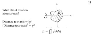
Mass and average value
Center of Mass
Example 1: For two equal masses, the center of mass is at the midpoint between them.
m1 = 1 m2 = 1
x1+x2
•
• x•
cm
• xcm = 2 .
x1 x2
Example 2: For unequal masses the center of mass is a weighted average of their positions.
m1 = 2 m2 = 1
2x1+x2
• x•
cm
• xcm = 3 .
x1 x2
In general, xcm = weighted average of position = �
mixi
.
mi
For a continuous density, δ(x), on the segment [a, b] (units of density are mass/unit length)
the sums become integrals. We will skip running through the logic of this since we are
about to show it for two dimensions.
� b
1
� b δ(x)
M = δ(x) dx, xcm = xδ(x) dx.
M a b
a a
In 2 dimensions we label the center of mass as (xcm, ycm) and we have the following formulas
1 1
M = δ(x, y) dA, xcm = xδ(x, y) dA, ycm = yδ(x, y) dA.
R M R M R
These formulas are easy to justify using our usual method for building integrals.
In this case, we divide our region into little pieces and we sum up the contributions of each
piece using an integral. To keep the figure below uncluttered we only show one piece and
we don’t bother to label it as the ith. In the end we will go directly to the integral, by
thinking if it as a sum.
y
x
��
��
dx
dy
•
(x, y), area = dA = dx dy
The little piece shown has mass δ(x, y) dA and the total mass is just the sum the pieces.
That is, it’s just the integral � �
M = δ dA.
R
Likewise the x and y coordinates of the center of mass are just the weighted average of the
x and y coordinates of each of the pieces. So, we get the formulas given above.

36. � �
� �
� �
Example: Suppose the unit square has density δ = xy; Find its mass and center of mass.
Answer:
� � � 1 � 1
1
M =
R
δ dA =
0 0
xy dx dy =
4
.
xcm =
1
M
� �
xδ dA =
1
M
� 1
0
� 1
0
x2
y dy dx.
��
1
2
This is easily computed as xcm = .
3 ��
By symmetry of the region and the density δ, we also have O 1
2
ycm =
3
.
Average Value
We can think of center of mass as the average position of the mass. That is, it’s the average
of position with respect to mass. We can also take averages of functions with respect to
other things. For instance, the average value of f(x, y) with respect to area on a region R is
1
f(x, y) dA.
area R R
In general, if we simply say the average value of a function, it means average value with
respect to area (or later, when we do triple integrals it can mean with respect to volume).
Example: What’s the average distance of a point in a unit square from the center?
Answer: We center the square on the origin. Notice each side has length 2a and the area
of the square is 4a2. So,
1
� � �
average distance = x2 + y2 dx dy.
4a2
square
By symmetry the integral is 8 times the integral of the triangular region R shown. We
actually compute the integral in polar coordinates.
8 y
average = r r dr dθ ��
4a2
R
� π/4 � a sec θ
=
2
r2
dr dθ
a2
0 0
� π/4 3 3 θ
2 a sec
= dθ
a2
0 3
a
= (
√
2 + ln(
√
2 + 1)).
3
x
��
a
a
r = a sec θ
��
R
This last integral was computed using integration by parts as
sec3
θ dθ =
sec θ dθ + sec θ tan θ
=
ln(sec θ + tan θ) + sec θ tan θ
.
2 2

37. Note: the center of mass is the average value of x and y with respect to mass.
The geometric center has coordinates given by the average value of x and y with respect to
area, i.e., the center of mass when δ = 1.

42. Problems: Mass and Average Value
Let R be the quarter of the unit circle in the first quadrant with density δ(x, y) = y.
1. Find the mass of R.
2. Find the center of mass.
3. Find the average distance from a point in R to the x axis.

43. Problems: Mass and Average Value
Let R be the quarter of the unit circle in the first quadrant with density δ(x, y) = y.
1. Find the mass of R.
Because R is a circular sector, it makes sense to use polar coordinates. The limits of
integration are then 0 ≤ r ≤ 1 and 0 ≤ θ ≤ π/2. In addition we have δ = r sin θ. To find
the mass of the region, we integrate the product of density and area.
M = δ dA
R
π/2 1
= (r sin θ) r dr dθ
0 0
π/2 1
= r2
sin θ dr dθ.
0 0
1 1 1
Inner: r3 sin θ = sin θ.
3 0 3
π/2 1
Outer: −1
3 cos θ 0
= 3.
The region has mass 1/3.
This seems like a reasonable conclusion – the region has area a little greater than 1/2 and
average density around 1/2.
2. Find the center of mass.
The center of mass (xcm, ycm) is described by
1 1
xcm =
M R
xδ dA and ycm =
M R
yδ dA.
From (1), M = 1
3.
1
xcm =
M R
xδ dA
π/2 1
= 3 (r cos θ)(r sin θ)r dr dθ
0 0
π/2 1
3
= 3r cos θ sin θ dr dθ.
0 0
3 4 1 3
Inner: r cos θ sin θ = cos θ sin θ.
4 0 4
π/2
3 1 3
Outer: (sin θ)2 = = xcm.
4 2 0 8
1

44. 1
ycm = yδ dA
M R
π/2 1
= 3 (r sin θ)(r sin θ)r dr dθ
0 0
π/2 1
= 3r3
sin2
θ dr dθ.
0 0
1
3 3
Inner: r4
sin2
θ = sin2
θ.
4 4
0
π/2
3 θ 1 3π
Outer: − sin(2θ) = = ycm.
4 2 4 16
0
3 3
The center of mass is at , ≈ (.4, .6).
8 4
This point is within R and agrees with our intuition that xcm < 1/2 and ycm > xcm.
3. Find the average distance from a point in R to the x axis.
1
To find the average of a function f(x, y) over an area, we compute f(x, y) dA.
Area R
Here f(x, y) = y.
π/2 1
1 1
y dA = (r sin θ)r dr dθ
Area π/4
R 0 0
π/2 1
4
= r2
sin θ dr dθ.
π 0 0
π/2 1
This should look familiar – we computed in (1) that r2
sin θ dr dθ =
1
. The average
3
0 0
4 1 4
distance from a point in R to the x axis is · = .
π 3 3π
2
ZZ
Z Z
Z Z

51. ZZ
ZZ Z Z
Z Z
Z Z

52. Moment of Inertia
Moment of inertia
We will leave it to your physics class to really explain what moment of inertia means. Very
briefly it measures an object’s resistance (inertia) to a change in its rotational motion. It is
analogous to the way mass measure the resistance to changes in the object’s linear motion.
Because it has to do with rotational motion the moment of inertia is always measured about
a reference line, which is thought of as the axis of rotation.
For a point mass, m, the moment of inertia about the line is
I = m d2
,
where d is the distance from the mass to the line. (The letter I is a standard notation for
moment of inertia.)
If we have a distributed mass we compute the moment of inertia by summing the contribu­
tions of each of its parts. If the mass has a continuous distribution, this sum is, of course,
an integral.
Example 1: Suppose the unit square, R, has density δ = xy.
Find its moment of inertia about the y-axis.
x
--
y
y
O 1
1
dx
dy
•
(x, y)
x
Answer: The distance from the small piece of the square (shown in the figure) to the y-axis
is x. If the piece has mass dm then its moment of inertia is
dI = x2
dm = x2
δ(x, y) dA = x3
y dx dy.
We took a shortcut here: we went straight to the notation for infinitesimal pieces, dI, dA
and used equalities. rather than using more formal notation ΔI, ΔA, using approximations
and then taking limits.
In the equation above, we used the notation dI to indicate it is just a small bit of moment
of inertia. We also used that the mass of a piece is density times area. Now it’s a simple
matter to sum up all the bits of moment of inertia using an integral
� � � 1 � 1
I = dI = x3
y dy dx =
1
.
8
R 0 0
(Note: this integral is so easy to compute that we don’t give the details.)
1

53. � � � �
Example 2: For the same square as in example 1, find the polar moment of inertia.
y
y
x
--
O 1
1
• (x, y)
r
Answer: The polar moment of inertia of a planar region is the moment of inertia about
the origin (the axis of rotation is the z-axis). Finding this is exactly the same as in example
1, except the distance to the axis is now the polar distance r. We get,
2 3
dI = r2
dm = (x + y2
)δ(x, y) dA = (x y + xy3
) dx dy.
Summing, using an integral gives
I =
R
dI =
1
0
1
0
x3
y + xy3
dy dx =
1
4
.
//
OO
Z Z Z Z
2

62. Moment of inertia
1. Let R be the triangle with vertices (0, 0), (1, 0), (1,
√
3) and density δ = 1. Find the
polar moment of inertia.

63. Moment of inertia
1. Let R be the triangle with vertices (0, 0), (1, 0), (1,
√
3) and density δ = 1. Find the
polar moment of inertia.
Answer: The region R is a 30, 60 , 90 triangle.
y
x
r
1
√
3
r = sec θ
The polar moment of inertia is the moment of inertia around the origin (that is, the z-axis).
The figure shows the triangle and a small square piece within R. If the piece has area dA
then its polar moment of inertia is dI = r2δ dA. Summing the contributions of all such
pieces and using δ = 1, dA = r dr dθ, we get the total moment of inertia is
�� �� ��
I = r2
δ dA = r2
r dr dθ = r3
dr dθ.
R R R
Next we find the limits of integration in polar coordinates. The line
x = 1 r cos θ = 1 r = sec θ.
⇔ ⇔
So, using radial stripes, the limits are: (inner) r from 0 to sec θ; (outer) θ from 0 to π/3.
Thus,
� π/3 � sec θ
I = r3
dr dθ.
0 0
sec4 θ
Inner integral: .
4
Outer integral: Use sec4 θ = sec2 θ sec2 θ = (1 + tan2 θ) d(tan θ) the outer integral is
⇒
1
�
tan θ +
tan3 θ
�
�
�
�π/3
=
1
�
√
3 +
(
√
3)3
�
=
√
3
.
4 3 �
0 4 3 2
√
3
The polar moment of inertia is .
2

64. � � � �
�
� �
� �
� �
� �
� �
Changing Variables in Multiple Integrals
1. Changing variables.
Double integrals in x, y coordinates which are taken over circular regions, or have inte­
grands involving the combination x2
+ y2
, are often better done in polar coordinates:
(1) f(x, y) dA = g(r, θ) r drdθ .
R R
This involves introducing the new variables r and θ, together with the equations relating
them to x, y in both the forward and backward directions:
(2) r = x2 + y2, θ = tan−1
(y/x); x = r cos θ, y = r sin θ .
Changing the integral to polar coordinates then requires three steps:
A. Changing the integrand f(x, y) to g(r, θ), by using (2);
B. Supplying the area element in the r, θ system: dA = r dr dθ ;
C. Using the region R to determine the limits of integration in the r, θ system.
In the same way, double integrals involving other types of regions or integrands can
sometimes be simplified by changing the coordinate system from x, y to one better adapted
to the region or integrand. Let’s call the new coordinates u and v; then there will be
equations introducing the new coordinates, going in both directions:
(3) u = u(x, y), v = v(x, y); x = x(u, v), y = y(u, v)
(often one will only get or use the equations in one of these directions). To change the
integral to u, v-coordinates, we then have to carry out the three steps A, B, C above. A
first step is to picture the new coordinate system; for this we use the same idea as for polar
coordinates, namely, we consider the grid formed by the level curves of the new coordinate
functions:
u=u0
u=u
(4) u(x, y) = u0, v(x, y) = v0 . 1
u=u2
Once we have this, algebraic and geometric intuition will usually handle
steps A and C, but for B we will need a formula: it uses a determinant v=v0
v=v
called the Jacobian, whose notation and definition are 1
v=v2
∂(x, y) � xu xv
�
(5) = .
∂(u, v) yu yv
Using it, the formula for the area element in the u, v-system is
�∂(x, y)�
�∂(u, v)�
(6) dA = du dv ,
1

65. � � � � � �
� �
� � � �
� � � �
� � � �
� � � �
� �
�
2 CHANGING VARIABLES IN MULTIPLE INTEGRALS
so the change of variable formula is
�∂(x, y)�
(7) f(x, y) dx dy = g(u, v) du dv ,
�∂(u, v)�
R R
where g(u, v) is obtained from f(x, y) by substitution, using the equations (3).
We will derive the formula (5) for the new area element in the next section; for now let’s
check that it works for polar coordinates.
Example 1. Verify (1) using the general formulas (5) and (6).
Solution. Using (2), we calculate:
∂(x, y)
=
xr xθ
=
cos θ −r sin θ
= r(cos2
θ + sin2
θ) = r ,
∂(r, θ) yr yθ sin θ r cos θ
so that dA = r dr dθ, according to (5) and (6); note that we can omit the absolute value,
since by convention, in integration problems we always assume r ≥ 0, as is implied already
by the equations (2).
We now work an example illustrating why the general formula is needed and how it is
used; it illustrates step C also — putting in the new limits of integration. 1
� � � �2
x − y -1
Example 2. Evaluate dx dy over the region R pictured.
x + y + 2
R
Solution. This would be a painful integral to work out in rectangular coordinates. -1
But the region is bounded by the lines
(8) x + y = ±1, x − y = ±1
and the integrand also contains the combinations x−y and x+y. These powerfully suggest
that the integral will be simplified by the change of variable (we give it also in the inverse
direction, by solving the first pair of equations for x and y):
u + v u − v
(9) u = x + y, v = x − y; x = , y = .
2 2
We will also need the new area element; using (5) and (9) above. we get
∂(x, y) � 1/2 1/2 � 1
(10) = � = − ;
∂(u, v) � 1/2 −1/2 � 2
note that it is the second pair of equations in (9) that were used, not the ones introducing
u and v. Thus the new area element is (this time we do need the absolute value sign in (6))
1
(11) dA = du dv .
2
We now combine steps A and B to get the new double integral; substituting into the
integrand by using the first pair of equations in (9), we get
� � � �2 � � � �2
x − y v 1
(12) dx dy = du dv .
x + y + 2 u + 2 2
R R
1

66. 3
CHANGING VARIABLES IN MULTIPLE INTEGRALS
In uv-coordinates, the boundaries (8) of the region are simply u = ±1, v = ±1, so the
integral (12) becomes
� � � �2 � 1 � 1 � �2
v 1 v 1
du dv = du dv
u + 2 2 u + 2 2
R −1 −1
We have
v2
�u=1
v2
v3
�1
2
= .
inner integral = − = ; outer integral =
2(u + 2) u=−1 3 9 −1 9

77. Problems: Change of Variables
Compute
ZZ
x + y
4
dx dy, where R is the square with vertices at (1, 0), (0, 1),
R 2 − x + y
(−1, 0) and (0, −1).

78. y v
y
v = 1
1
v ˜
= −1 u = 1 u = 1
R u = 1
R R
−
x x u
−1 1
u = −1 v = −1
−1
v = −1
Problems: Change of Variables
4
x + y
Compute dx dy, where R is the square with vertices at (1, 0), (0, 1),
R 2
( 1, 0) and (0, 1).
− x + y
− −
Answer: Since the region is bounded by the lines x + y = ±1 and x − y = ±1, we make a
change of variables:
u = x + y v = x − y.
∂(u, v) ∂(x, y)
Computing the Jacobian: = = 1
∂(x, y)
−2 ⇒ /2.
∂(u, v)
−
1
Thus, dx dy = du dv.
2
Using either method 1 or method 2 we see the boundaries are given by u = ±1, v = ±1 ⇒
x 4
+ 4
y 1 1
u
1
the integral is dx dy = du dv.
R w − x + y 2 v 2
−1 −1 −
u5
u=1
1
Inner integral =
= .
10(2 − v)4 4
u= 5(2 − v
−1 )
1
1 26
Outer integral =
=
.06.
15(2 − v)3
1 405
≈
−
We’re integrating the fourth power of a fraction whose numerator ranges between −1 and
1 and whose denominator ranges between 1 and 3. The value of this integrand will always
be positive and will often be small, so this answer seems reasonable.
y y
y
-- --
--

79. � � � �
� � � �
� � � �
� �
� �
� �
�
� �
� �
� �
�
x
Changing Variables in Multiple Integrals
dA
dθ
y
rd θ
2. The area element.
dr
In polar coordinates, we found the formula dA = r dr dθ for the area element by
drawing the grid curves r = r0 and θ = θ0 for the r, θ-system, and determining (see
the picture) the infinitesimal area of one of the little elements of the grid.
For general u, v-coordinates, we do the same thing. The grid curves (4) divide up the
plane into small regions ΔA bounded by these contour curves. If the contour curves are close
together, they will be approximately parallel, so that the grid element will be approximately
a small parallelogram, and y
(13) ΔA ≈ area of parallelogram PQRS = |PQ × PR|
In the uv-system, the points P, Q, R have the coordinates
P : (u0, v0), Q : (u0 + Δu, v0), R : (u0, v0 + Δv) ;
to use the cross-product however in (13), we need PQ and PR in i j - coordinates.
Consider PQ first; we have
(14) PQ = Δx i + Δy j ,
v=v 0 + Δv
S
v=v0
R ΔA
Q u=u0 +Δ u
P u=u0
x
where Δx and Δy are the changes in x and y as you hold v = v0 and change u0 to u0 + Δu.
According to the definition of partial derivative,
∂x ∂y
Δx ≈ Δu, Δy ≈ Δu;
∂u ∂u
0 0
so that by (14),
∂x ∂y
(15) PQ ≈ Δu i + Δu j .
∂u ∂u
0 0
In the same way, since in moving from P to R we hold u fixed and increase v0 by Δv,
∂x ∂y
(16) PR ≈ Δv i + Δv j .
∂v ∂v
0 0
We now use (13); since the vectors are in the xy-plane, PQ × PR has only a k -component,
and we calculate from (15) and (16) that
� xuΔu yuΔu �
k -component of PQ × PR ≈ � xv yv
�
Δv Δv 0
� x x �
(17) = � u v
ΔuΔv ,
� y y �
u v 0
where we have first taken the transpose of the determinant (which doesn’t change its value),
and then factored the Δu and Δv out of the two columns. Finally, taking the absolute
value, we get from (13) and (17), and the definition (5) of Jacobian,
�∂(x, y)�
�∂(u, v)�
0
ΔA ≈ ΔuΔv ;
passing to the limit as Δu, Δv → 0 and dropping the subscript 0 (so that P becomes any
point in the plane), we get the desired formula for the area element,
�∂(x, y)�
�∂(u, v)�
dA = � du dv .
1

83. Problems: Polar Coordinates and the Jacobian
p 1 y ∂(r, θ) 1
1. Let r = x2 + y2 and θ = tan−
. Directly calculate the Jacobian = .
x ∂(x, y) r
2. For the change of variables x = u, y =
√
r2 − u2, write dx dy in terms of u and r.

84. Problems: Polar Coordinates and the Jacobian
1. Let r =
x
.
−1 y ∂(r, θ) 1
2 + y2 and θ = tan . Directly calculate the Jacobian =
∂(x, y)
x
r
Answer: Because we are familiar with the change of variables from rectangular to polar
∂(r, θ) ∂(x, y)
coordinates and we know that · = 1, this result should not come as a surprise.
∂(x, y) ∂(r, θ)
∂(r, θ)
rx ry
=
θx θy
∂(x, y)
2x 2y
√ √
2 2
2 x2+y 2 x2+y
−y/x2 1/x
=
1+(y/x)2
x √ y
√
1+(y/x)2
2 2
x2+y x2+y
=
− y
2
x
2+y 2
2+y
x x
x y
r r
=
− y x
2 2
r r
x2 + y2 1
= = .
3
r r
√
For the change of variables x = u, y = r2 − u2, write dx dy in terms of u and r.
2.
∂(x, y)
Answer: We know dx dy =
du dr.
∂(u, r)
∂(x, y)
xu xr
=
∂(u, r)
yu yr
1 0
−u
√ √ r
r2−u2 r2−u2
r
=
= √
2 − u2
r
r
Hence dx dy = √ du dr.
r2 − u2

85. Z Z Z Z

97. Z Z