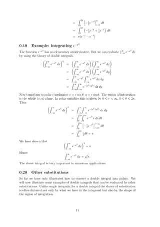
This document provides examples and explanations of double integrals. It defines a double integral as integrating a function f(x,y) over a region R in the xy-plane. It then gives three key points: 1) To evaluate a double integral, integrate the inner integral first treating the other variable as a constant, then integrate the outer integral. 2) The easiest regions to integrate over are rectangles, as the limits of integration will all be constants. 3) For non-rectangular regions, the limits of integration may be variable, requiring more careful analysis to determine the limits for each integral.

1. Double integrals
Notice: this material must not be used as a substitute for attending
the lectures
1

2. 0.1 What is a double integral?
Recall that a single integral is something of the form
b
f (x) dx
a
A double integral is something of the form
f (x, y) dx dy
R
where R is called the region of integration and is a region in the (x, y) plane. The
double integral gives us the volume under the surface z = f (x, y), just as a single
integral gives the area under a curve.
0.2 Evaluation of double integrals
To evaluate a double integral we do it in stages, starting from the inside and working
out, using our knowledge of the methods for single integrals. The easiest kind of
region R to work with is a rectangle. To evaluate
f (x, y) dx dy
R
proceed as follows:
• work out the limits of integration if they are not already known
• work out the inner integral for a typical y
• work out the outer integral
0.3 Example
Evaluate
2 3
(1 + 8xy) dx dy
y=1 x=0
3
Solution. In this example the “inner integral” is x=0 (1 + 8xy) dx with y treated as a
constant.
 
2 3
 
 
integral = 
 (1 + 8xy) dx 
 dy
y=1  x=0 
work out treating y as constant
3
2 8x2 y
= x+ dy
y=1 2 x=0
2
= (3 + 36y) dy
y=1
2

3. 2
36y 2
= 3y +
2 y=1
= (6 + 72) − (3 + 18)
= 57
0.4 Example
Evaluate
π/2 1
y sin x dy dx
0 0
Solution.
π/2 1
integral = y sin x dy dx
0 0
1
π/2 y2
= sin x dx
0 2 y=0
π/2
1
= 2
sin x dx
0
π/2
1 1
= − 2 cos x = 2
x=0
0.5 Example
Find the volume of the solid bounded above by the plane z = 4 − x − y and below
by the rectangle R = {(x, y) : 0 ≤ x ≤ 1 0 ≤ y ≤ 2}.
Solution. The volume under any surface z = f (x, y) and above a region R is given by
V = f (x, y) dx dy
R
In our case
2 1
V = (4 − x − y) dx dy
0 0
2 1 2
= 4x − 1 x2 − yx
2
dy = 1
(4 − 2 − y) dy
0 x=0 0
2
7y y 2
= − = (7 − 2) − (0) = 5
2 2 y=0
The double integrals in the above examples are the easiest types to evaluate because
they are examples in which all four limits of integration are constants. This happens
when the region of integration is rectangular in shape. In non-rectangular regions
of integration the limits are not all constant so we have to get used to dealing with
non-constant limits. We do this in the next few examples.
3

4. 0.6 Example
Evaluate
2 x
y 2 x dy dx
0 x2
Solution.
2 x
integral = y 2 x dy dx
0 x2
y=x
2 y3x
= dx
0 3 y=x2
2
x4 x7 2 x5 x8
= − dx = −
0 3 3 15 24 0
32 256 128
= − =−
15 24 15
0.7 Example
Evaluate
π x2 1 y
cos dy dx
π/2 0 x x
1
Solution. Recall from elementary calculus the integral cos my dy = m
sin my for m
independent of y. Using this result,
2
y y=x
 
π1 sin x 
integral =  dx
π/2 x 1
x y=0
π
= sin x dx = [− cos x]π
x=π/2 = 1
π/2
0.8 Example
Evaluate √
4 y √
ex/ y
dx dy
1 0
Solution.
√ √
x= y
4ex/ y
integral = √ dy
1 1/ y x=0
4 √ √ 4
= ( ye − y) dy = (e − 1) y 1/2 dy
1 1
3/2 4
y 2
= (e − 1) = (e − 1)(8 − 1)
3/2 y=1
3
14
= (e − 1)
3
4

5. 0.9 Evaluating the limits of integration
When evaluating double integrals it is very common not to be told the limits of
integration but simply told that the integral is to be taken over a certain specified
region R in the (x, y) plane. In this case you need to work out the limits of integration
for yourself. Great care has to be taken in carrying out this task. The integration
can in principle be done in two ways: (i) integrating first with respect to x and then
with respect to y, or (ii) first with respect to y and then with respect to x. The
limits of integration in the two approaches will in general be quite different, but both
approaches must yield the same answer. Sometimes one way round is considerably
harder than the other, and in some integrals one way works fine while the other leads
to an integral that cannot be evaluated using the simple methods you have been
taught. There are no simple rules for deciding which order to do the integration in.
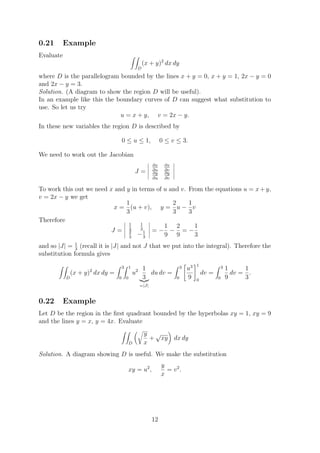
0.10 Example
Evaluate
(3 − x − y) dA [dA means dxdy or dydx]
D
where D is the triangle in the (x, y) plane bounded by the x-axis and the lines y = x
and x = 1.
Solution. A good diagram is essential.
Method 1 : do the integration with respect to x first. In this approach we select a typical
y value which is (for the moment) considered fixed, and we draw a horizontal
line across the region D; this horizontal line intersects the y axis at the typical
y value. Find out the values of x (they will depend on y) where the horizontal
line enters and leaves the region D (in this problem it enters at x = y and
leaves at x = 1). These values of x will be the limits of integration for the inner
integral. Then you determine what values y has to range between so that the
horizontal line sweeps the entire region D (in this case y has to go from 0 to 1).
This determines the limits of integration for the outer integral, the integral with
respect to y. For this particular problem the integral becomes
1 1
(3 − x − y) dA = (3 − x − y) dx dy
D 0 y
x=1
1 x2
= 3x − − yx dy
0 2 x=y
1 y2
= 3 − 1 − y − 3y −
2
− y2 dy
0 2
y=1
5 1 3 5y y3
= − 4y + y 2 dy = − 2y 2 +
0 2 2 2 2 y=0
5 1
= −2+ =1
2 2
5

6. Method 2 : do the integration with respect to y first and then x. In this approach we
select a “typical x” and draw a vertical line across the region D at that value
of x.
Vertical line enters D at y = 0 and leaves at y = x. We then need to let x
go from 0 to 1 so that the vertical line sweeps the entire region. The integral
becomes
1 x
(3 − x − y) dA = (3 − x − y) dy dx
D 0 0
y=x
1 y2
= 3y − xy − dx
0 2 y=0
1 x2 1 3x2
= 3x − x2 − dx = 3x − dx
0 2 0 2
1
3x2 x3
= − =1
2 2 x=0
Note that Methods 1 and 2 give the same answer. If they don’t it means something
is wrong.
0.11 Example
Evaluate
(4x + 2) dA
D
where D is the region enclosed by the curves y = x2 and y = 2x.
Solution. Again we will carry out the integration both ways, x first then y, and then
vice versa, to ensure the same answer is obtained by both methods.
Method 1 : We do the integration first with respect to x and then with respect to y. We
shall need to know where the two curves y = x2 and y = 2x intersect. They
intersect when x2 = 2x, i.e. when x = 0, 2. So they intersect at the points (0, 0)
and (2, 4).
√
For a typical y, the horizontal line will enter D at x = y/2 and leave at x = y.
Then we need to let y go from 0 to 4 so that the horizontal line sweeps the
entire region. Thus
√
4 x= y
(4x + 2) dA = (4x + 2) dx dy
D 0 x=y/2
√
4 x= y 4 √ y2
= 2x2 + 2x dy = (2y + 2 y) − +y dy
0 x=y/2 0 2
4
4
1/2 y2 y 2 2y 3/2 y 3
= y + 2y − dy = + − =8
0 2 2 3/2 6 0
6

7. Method 2 : Integrate first with respect to y and then x, i.e. draw a vertical line across D
at a typical x value. Such a line enters D at y = x2 and leaves at y = 2x. The
integral becomes
2 2x
(4x + 2) dA = (4x + 2) dy dx
D 0 x2
2
= [4xy + 2y]y=2x dx
y=x2
0
2
= 8x2 + 4x − 4x3 + 2x2 dx
0
2 2
= (6x2 − 4x3 + 4x) dx = 2x3 − x4 + 2x2 =8
0 0
The example we have just done shows that it is sometimes easier to do it one way
than the other. The next example shows that sometimes the difference in effort is
more considerable. There is no general rule saying that one way is always easier than
the other; it depends on the individual integral.
0.12 Example
Evaluate
(xy − y 3 ) dA
D
where D is the region consisting of the square {(x, y) : −1 ≤ x ≤ 0, 0 ≤ y ≤ 1}
together with the triangle {(x, y) : x ≤ y ≤ 1, 0 ≤ x ≤ 1}.
Method 1 : (easy). integrate with respect to x first. A diagram will show that x goes
from −1 to y, and then y goes from 0 to 1. The integral becomes
1 y
(xy − y 3 ) dA = (xy − y 3 ) dx dy
D 0 −1
1 x2 x=y
3
= y − xy dy
0 2 x=−1
1 y3
= − y 4 − ( 2 y + y 3 ) dy
1
0 2
1
1 y3 y4 y5 y2 23
= − − y4 − 2 y
1
dy = − − − =−
0 2 8 5 4 y=0
40
Method 2 : (harder). It is necessary to break the region of integration D into two sub-
regions D1 (the square part) and D2 (triangular part). The integral over D is
given by
(xy − y 3 ) dA = (xy − y 3 ) dA + (xy − y 3 ) dA
D D1 D2
7

8. c b c
which is the analogy of the formula a f (x) dx = a f (x) dx + b f (x) dx for
single integrals. Thus
0 1 1 1
(xy − y 3 ) dA = (xy − y 3 ) dy dx + (xy − y 3 ) dy dx
D −1 0 0 x
1 1
0 xy 2 y 4 1 xy 2 y 4
= − dx + − dx
−1 2 4 y=0 0 2 4 y=x
3
0
1 1 1 x 1 x x4
= 2
x − dx + − − − dx
−1 4 0 2 4 2 4
0 1
x2 x x2 x x4 x5
= − + − − +
4 4 −1 4 4 8 20 0
3 23
= −1 −
2
=−
40 40
In the next example the integration can only be done one way round.
0.13 Example
Evaluate
sin x
dA
D x
where D is the triangle {(x, y) : 0 ≤ y ≤ x, 0 ≤ x ≤ π}.
Solution. Let’s try doing the integration first with respect to x and then y. This gives
sin x π π sin x
dA = dx dy
D x 0 y x
but we cannot proceed because we cannot find an indefinite integral for sin x/x. So,
let’s try doing it the other way. We then have
sin x π
sin x x
dA = dy dx
D x 0 0 x
π sin x x π
= y dx = sin x dx
0 x y=0 0
= [− cos x]π = 1 − (−1) = 2
0
0.14 Example
Find the volume of the tetrahedron that lies in the first octant and is bounded by the
three coordinate planes and the plane z = 5 − 2x − y.
Solution. The given plane intersects the coordinate axes at the points ( 5 , 0, 0), (0, 5, 0)
2
and (0, 0, 5). Thus, we need to work out the double integral
(5 − 2x − y) dA
D
8

9. where D is the triangle in the (x, y) plane with vertices (x, y) = (0, 0), ( 5 , 0) and
2
(0, 5). It is a good idea to draw another diagram at this stage showing just the region
5
D in the (x, y) plane. Note that the equation of the line joining the points ( 2 , 0) and
(0, 5) is y = −2x + 5. Then:
5 (5−y)/2
volume = (5 − 2x − y) dA = (5 − 2x − y) dx dy
D 0 0
5 x=(5−y)/2
= 5x − x2 − yx dy
0 x=0
2
5 5−y 5−y 5−y
= 5 − −y dy
0 2 2 2
5 2
25 5y y
= − + dy
0 4 2 4
5
25y 5y 2 y 3 125
= − + =
4 4 12 0
12
0.15 Changing variables in a double integral
We know how to change variables in a single integral:
b B dx
f (x) dx = f (x(u)) du
a A du
where A and B are the new limits of integration.
For double integrals the rule is more complicated. Suppose we have
f (x, y) dx dy
D
and want to change the variables to u and v given by x = x(u, v), y = y(u, v). The
change of variables formula is
f (x, y) dx dy = f (x(u, v), y(u, v))|J| du dv (0.1)
D D∗
where J is the Jacobian, given by
∂x ∂y ∂x ∂y
J= −
∂u ∂v ∂v ∂u
and D∗ is the new region of integration, in the (u, v) plane.
0.16 Transforming a double integral into polars
A very commonly used substitution is conversion into polars. This substitution is
particularly suitable when the region of integration D is a circle or an annulus (i.e.
region between two concentric circles). Polar coordinates r and θ are defined by
x = r cos θ, y = r sin θ
9

10. The variables u and v in the general description above are r and θ in the polar
coordinates context and the Jacobian for polar coordinates is
∂x ∂y ∂x ∂y
J = −
∂r ∂θ ∂θ ∂r
= (cos θ)(r cos θ) − (−r sin θ)(sin θ)
= r(cos2 θ + sin2 θ) = r
So |J| = r and the change of variables rule (0.1) becomes
f (x, y) dx dy = f (r cos θ, r sin θ) r dr dθ
D D∗
0.17 Example
Use polar coordinates to evaluate
xy dx dy
D
where D is the portion of the circle centre 0, radius 1, that lies in the first quadrant.
Solution. For the portion in the first quadrant we need 0 ≤ r ≤ 1 and 0 ≤ θ ≤ π/2.
These inequalities give us the limits of integration in the r and θ variables, and these
limits will all be constants.
With x = r cos θ, y = r sin θ the integral becomes
π/2 1
xy dx dy = r2 cos θ sin θ r dr dθ
D 0 0
1
r4 π/2
= cos θ sin θ dθ
0 4 r=0
π/2 1 π/2 1
= sin θ cos θ dθ = sin 2θ dθ
0 4 0 8
π/2
1 cos 2θ 1
= − =
8 2 0
8
0.18 Example
Evaluate
2 +y 2 )
e−(x dx dy
D
where D is the region between the two circles x2 + y 2 = 1 and x2 + y 2 = 4.
Solution. It is not feasible to attempt this integral by any method other than trans-
forming into polars.
Let x = r cos θ, y = r sin θ. In terms of r and θ the region D between the two circles
is described by 1 ≤ r ≤ 2, 0 ≤ θ ≤ 2π, and so the integral becomes
2 +y 2 )
2π 2 2
e−(x dx dy = e−r r dr dθ
D 0 1
10

11. 2π 2 2
= − 1 e−r
2
dθ
0 r=1
2π
= − 2 e−4 + 2 e−1 dθ
1 1
0
= π(e−1 − e−4 )
2
0.19 Example: integrating e−x
2 ∞ −x2
The function e−x has no elementary antiderivative. But we can evaluate −∞ e dx
by using the theory of double integrals.
∞ 2 ∞ ∞
2 2 2
e−x dx = e−x dx e−x dx
−∞ −∞ −∞
∞ ∞
−x2 2
= e dx e−y dy
−∞ −∞
∞ ∞
−y 2 −x2
= e e dx dy
−∞ −∞
∞ ∞ 2 +y 2 )
= e−(x dx dy
−∞ −∞
Now transform to polar coordinates x = r cos θ, y = r sin θ. The region of integration
is the whole (x, y) plane. In polar variables this is given by 0 ≤ r < ∞, 0 ≤ θ ≤ 2π.
Thus
∞ 2 ∞ ∞
2 2 +y 2 )
e−x dx = e−(x dx dy
−∞ −∞ −∞
2π ∞ 2
= e−r r dr dθ
0 0
2π 2 r=∞
= − 1 e−r
2
dθ
0 r=0
2π
1
= 2
dθ =π
0
We have shown that
∞ 2
2
e−x dx =π
−∞
Hence ∞ √
2
e−x dx = π.
−∞
The above integral is very important in numerous applications.
0.20 Other substitutions
So far we have only illustrated how to convert a double integral into polars. We
will now illustrate some examples of double integrals that can be evaluated by other
substitutions. Unlike single integrals, for a double integral the choice of substitution
is often dictated not only by what we have in the integrand but also by the shape of
the region of integration.
11

12. 0.21 Example
Evaluate
(x + y)2 dx dy
D
where D is the parallelogram bounded by the lines x + y = 0, x + y = 1, 2x − y = 0
and 2x − y = 3.
Solution. (A diagram to show the region D will be useful).
In an example like this the boundary curves of D can suggest what substitution to
use. So let us try
u = x + y, v = 2x − y.
In these new variables the region D is described by
0 ≤ u ≤ 1, 0 ≤ v ≤ 3.
We need to work out the Jacobian
∂x ∂x
J= ∂u ∂v
∂y ∂y
∂u ∂v
To work this out we need x and y in terms of u and v. From the equations u = x + y,
v = 2x − y we get
1 2 1
x = (u + v), y = u − v
3 3 3
Therefore
1 1 1 2 1
J = 3 31 = − − = −
2
3
−3 9 9 3
and so |J| = 1 (recall it is |J| and not J that we put into the integral). Therefore the
3
substitution formula gives
1
2
3 1
2 1 3 u3 3 1 1
(x + y) dx dy = u du dv = dv = dv = .
D 0 0 3 0 9 0 0 9 3
=|J|
0.22 Example
Let D be the region in the first quadrant bounded by the hyperbolas xy = 1, xy = 9
and the lines y = x, y = 4x. Evaluate
y √
+ xy dx dy
D x
Solution. A diagram showing D is useful. We make the substitution
y
xy = u2 , = v2.
x
12

13. We will need x and y in terms of u and v. By multiplying the above equations we
get y 2 = u2 v 2 . Hence y = uv and x = u/v. In the (u, v) variables the region D is
described by
1 ≤ u ≤ 3, 1 ≤ v ≤ 2.
The Jacobian is
∂x ∂x 1
∂u ∂v v
− vu2 u u 2u
J= ∂y ∂y = = + =
∂u ∂v
v u v v v
Therefore
y √
+ xy dx dy
D x
2 3 2u
= (v + u)|J| du dv = (v + u)
du dv
1 1 v
u=3
2 3 2u2 2
2 2u3
= 2u + du dv = u + dv
1 1 v 1 3v u=1
2 2
18 2 52 52
= 9+ − 1+ dv = 8v + ln v = 8 + ln 2.
1 v 3v 3 1 3
0.23 Application of double integrals: centres of gravity
We will show how double integrals may be used to find the location of the centre
of gravity of a two-dimensional object. Mathematically speaking, a plate is a thin
2-dimensional distribution of matter considered as a subset of the (x, y) plane. Let
σ = mass per unit area
This is the definition of density for two-dimensional objects. If the plate is all made
of the same material (a sheet of metal, perhaps) then σ would be a constant, the value
of which would depend on the material of which the plate is made. However, if the
plate is not all made of the same material then σ could vary from point to point on
the plate and therefore be a function of x and y, σ(x, y). For some objects, part of the
object may be made of one material and part of it another (some currencies have coins
that are like this). But σ(x, y) could quite easily vary in a much more complicated
way (a pizza is a simple example of an object with an uneven distribution of matter).
The intersection of the two thin strips defines a small rectangle of length δx and width
δy. Thus
mass of little rectangle = (mass per unit area)(area)
= σ(x, y) dx dy
Therefore the total mass of the plate D is
M= σ(x, y) dx dy.
D
Suppose you try to balance the plate D on a pin. The centre of mass of the plate is
the point where you would need to put the pin. It can be shown that the coordinates
13

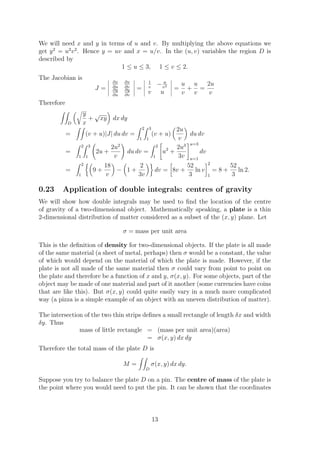
14. (¯, y ) of the centre of mass are given by
x ¯
x σ(x, y) dA y σ(x, y) dA
D D
x=
¯ , y=
¯ (0.2)
σ(x, y) dA σ(x, y) dA
D D
0.24 Example
A homogeneous triangle with vertices (0, 0), (1, 0) and (1, 3). Find the coordinates of
its centre of mass.
[‘Homogeneous’ means the plate is all made of the same material which is uniformly
distributed across it, so that σ(x, y) = σ, a constant.]
Solution. A diagram of the triangle would be useful. With σ constant, we have
1 3x 1
σx dA σ x dy dx [xy]y=3x dx
y=0
D 0 0 0
x =
¯ = 1 3x = 1
σ dA σ dy dx [y]y=3x dx
y=0
D 0 0 0
1
3x2 dx 1 2
0
= 1 = =
3/2 3
3x dx
0
and
y=3x
1 3x
1 y2
σy dA σ y dy dx dx
D 0 0
0 2 y=0
y =
¯ = 1 3x = 1
σ dA σ dy dx [y]y=3x dx
y=0
D 0 0 0
1 9x2
dx 3/2
= 0 2 = = 1.
1
3/2
3x dx
0
2
So the centre of mass is at (¯, y ) = ( 3 , 1).
x ¯
0.25 Example
Find the centre of mass of a circle, centre the origin, radius 1, if the right half is made
of material twice as heavy as the left half.
Solution. By symmetry, it is clear that the centre of mass will be somewhere on the
x-axis, and so y = 0. In order to model the fact that the right half is twice as heavy,
¯
we can take
2σ x > 0
σ(x, y) =
σ x<0
with the σ in the right hand side of the above expression being any positive constant.
14

15. From the general formula,
x σ(x, y) dA
D
x=
¯ . (0.3)
σ(x, y) dA
D
Let us work out the integral in the numerator first. We shall need to break it up as
follows
xσ(x, y) dA = + = 2σx dA + σx dA
D right half left half right left
The circular geometry suggests we convert to plane polars, x = r cos θ, y = r sin θ.
Recall that, in this coordinate system, dA = r dr dθ. The right half of the circle
is described by −π/2 ≤ θ ≤ π/2, 0 ≤ r ≤ 1, and the left half similarly but with
π/2 ≤ θ ≤ 3π/2. Thus
π/2 1 3π/2 1
xσ(x, y) dA = 2σ(r cos θ) r dr dθ + σ(r cos θ) r dr dθ
D −π/2 0 π/2 0
r=1 r=1
π/2 r3 3π/2 r3
= 2σ cos θ dθ + σ cos θ dθ
−π/2 3 r=0 π/2 3 r=0
2σ π/2 σ 3π/2
= cos θ dθ + cos θ dθ
3 −π/2 3 π/2
4σ 2σ 2σ
= − = .
3 3 3
Finally, we work out the denominator in (0.3):
σ(x, y) dA = σ dA + 2σ dA
D left half right half
= σ dA + 2σ dA
left half right half
= σ(area of left half) + 2σ(area of right half)
= σ(π/2) + 2σ(π/2)
3σπ
=
2
Therefore the x coordinate of the centre of mass of the object is
2σ/3 4
x=
¯ = .
3σπ/2 9π
15