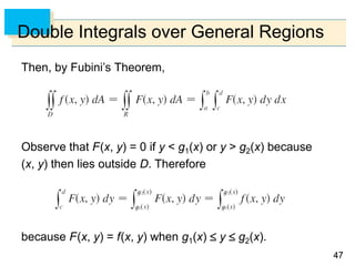
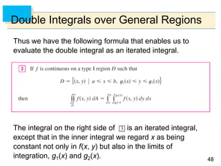
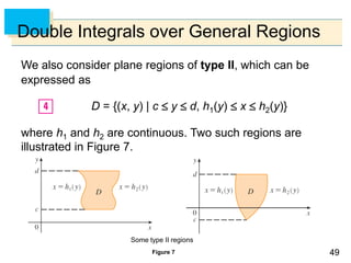
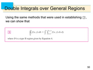
This document provides an overview of double integrals and their use in calculating volumes. It begins by reviewing definite integrals of single-variable functions. It then introduces double integrals, which can be used to calculate the volume of a solid under a surface defined by a two-variable function f(x,y). This is done by dividing the domain into subrectangles and approximating the volume as a double Riemann sum. Several examples are provided to demonstrate calculating volumes and average values over a region using double integrals. The document also discusses double integrals over non-rectangular regions and provides formulas for calculating them using iterated integrals for specific region types.

![44
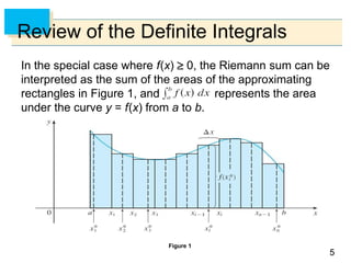
Review of the Definite Integrals
First let’s recall the basic facts concerning definite integrals
of functions of a single variable.
If f(x) is defined for a x b, we start by dividing the
interval [a, b] into n subintervals [xi–1, xi] of equal width
x = (b – a)/n and we choose sample points in these
subintervals. Then we form the Riemann sum
and take the limit of such sums as n → to obtain the
definite integral of f from a to b:](https://image.slidesharecdn.com/chatper15-191003195240/85/Chatper-15-4-320.jpg)

![77
In a similar manner we consider a function f of two
variables defined on a closed rectangle
R = [a, b] [c, d] = {(x, y) |a x b, c y d}
and we first suppose that f(x, y) 0.
The graph of f is a surface
with equation z = f(x, y).
Let S be the solid that lies
above R and under the
graph of f, that is,
S = {(x, y, z) |0 z f(x, y), (x, y) R}
(See Figure 2.)
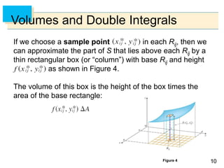
Volumes and Double Integrals
Figure 2](https://image.slidesharecdn.com/chatper15-191003195240/85/Chatper-15-7-320.jpg)
![88
Volumes and Double Integrals
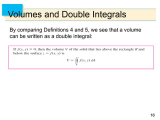
Our goal is to find the volume of S.
The first step is to divide the rectangle R into
subrectangles.
We accomplish this by dividing the interval [a, b] into m
subintervals [xi – 1, xi] of equal width x = (b – a)/m and
dividing [c, d ] into n subintervals [yj – 1, yj] of equal width
y = (d – c)/n.](https://image.slidesharecdn.com/chatper15-191003195240/85/Chatper-15-8-320.jpg)
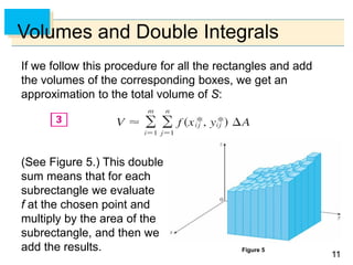
![99
Volumes and Double Integrals
By drawing lines parallel to the coordinate axes through the
endpoints of these subintervals, as in Figure 3, we form the
subrectangles
Rij = [xi–1, xi] [yj–1, yj] = {(x, y) | xi–1 x xi, yj–1 y yj}
each with area A = x y.
Figure 3
Dividing R into subrectangles](https://image.slidesharecdn.com/chatper15-191003195240/85/Chatper-15-9-320.jpg)
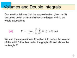
![1414
Volumes and Double Integrals
It is shown in courses on advanced calculus that all
continuous functions are integrable. In fact, the double
integral of f exists provided that f is “not too discontinuous.”
In particular, if f is bounded [that is, there is a constant M
such that |f(x, y)| M for all (x, y) in R], and f is continuous
there, except on a finite number of smooth curves, then f is
integrable over R.](https://image.slidesharecdn.com/chatper15-191003195240/85/Chatper-15-14-320.jpg)
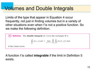
![1515
Volumes and Double Integrals
The sample point can be chosen to be any point
in the subrectangle Rij, but if we choose it to be the upper
right-hand corner of Rij [namely (xi, yj), see Figure 3], then
the expression for the double integral looks simpler:
Figure 3
Dividing R into subrectangles](https://image.slidesharecdn.com/chatper15-191003195240/85/Chatper-15-15-320.jpg)
![1717
Volumes and Double Integrals
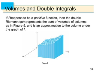
The sum in Definition 5,
is called a double Riemann sum and is used as an
approximation to the value of the double integral. [Notice
how similar it is to the Riemann sum in for a function of
a single variable.]](https://image.slidesharecdn.com/chatper15-191003195240/85/Chatper-15-17-320.jpg)
![1919
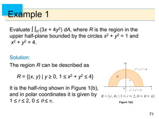
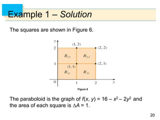
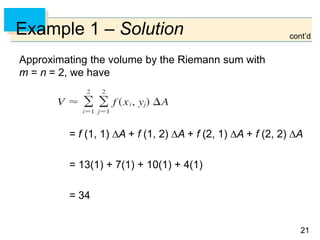
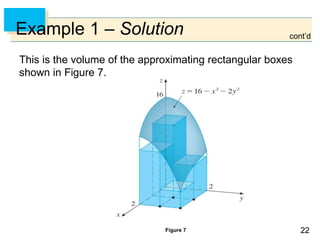
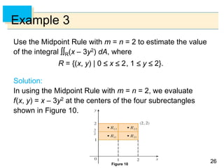
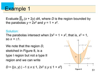
Example 1
Estimate the volume of the solid that lies above the square
R = [0, 2] [0, 2] and below the elliptic paraboloid
z = 16 – x2 – 2y2.
Divide R into four equal squares and choose the sample
point to be the upper right corner of each square Rij.
Sketch the solid and the approximating
rectangular boxes.](https://image.slidesharecdn.com/chatper15-191003195240/85/Chatper-15-19-320.jpg)

![2424
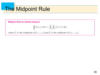
The Midpoint Rule
The methods that we used for approximating single
integrals (the Midpoint Rule, the Trapezoidal Rule,
Simpson’s Rule) all have counterparts for double integrals.
Here we consider only the Midpoint Rule for double
integrals.
This means that we use a double Riemann sum to
approximate the double integral, where the sample point
in Rij is chosen to be the center of Rij. In
other words, is the midpoint of [xi–1, xi] and is the
midpoint of [yj–1, yj].](https://image.slidesharecdn.com/chatper15-191003195240/85/Chatper-15-24-320.jpg)
![3030
Average Values
Recall that the average value of a function f of one variable
defined on an interval [a, b] is
In a similar fashion we define the average value of a
function f of two variables defined on a rectangle R to be
where A(R) is the area of R.](https://image.slidesharecdn.com/chatper15-191003195240/85/Chatper-15-30-320.jpg)
![3131
Average Values
If f(x, y) 0, the equation
A(R) fave = f(x, y) dA
says that the box with base R and height fave has the same
volume as the solid that lies under the graph of f.
[If z = f(x, y) describes a
mountainous region and you
chop off the tops of the
mountains at height fave, then
you can use them to fill in the
valleys so that the region
becomes completely flat.
See Figure 11.] Figure 11](https://image.slidesharecdn.com/chatper15-191003195240/85/Chatper-15-31-320.jpg)
![3535
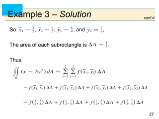
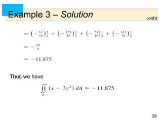
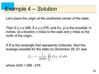
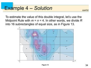
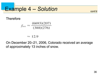
Example 4 – Solution
The area of each subrectangle is
Using the contour map to estimate the value of f at the
center of each subrectangle, we get
≈ A[0 + 15 + 8 + 7 + 2 + 25 + 18.5
+ 11 + 4.5 + 28 + 17 + 13.5 + 12
+ 15 + 17.5 + 13]
= (6693)(207)
= 6693 mi2
cont’d](https://image.slidesharecdn.com/chatper15-191003195240/85/Chatper-15-35-320.jpg)

![3838
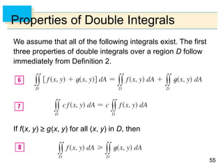
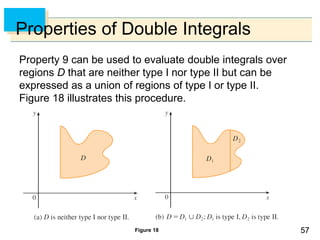
Properties of Double Integrals
We list here three properties of double integrals. We
assume that all of the integrals exist. Properties 7 and 8 are
referred to as the linearity of the integral.
[f(x, y) + g(x, y)] dA = f(x, y) dA + g(x, y) dA
c f(x, y) dA = c f(x, y) dA where c is a constant
If f(x, y) g(x, y) for all (x, y) in R, then
f(x, y) dA g(x, y) dA](https://image.slidesharecdn.com/chatper15-191003195240/85/Chatper-15-38-320.jpg)
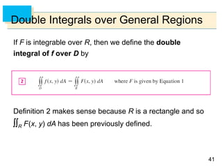
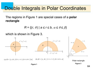
![4545
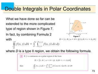
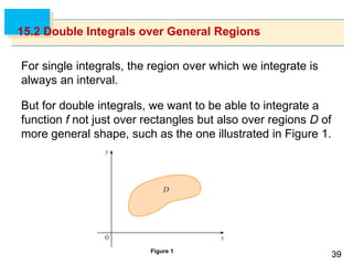
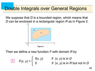
Double Integrals over General Regions
A plane region D is said to be of type I if it lies between the
graphs of two continuous functions of x, that is,
D = {(x, y) | a x b, g1(x) y g2(x)}
where g1 and g2 are continuous on [a, b]. Some examples
of type I regions are shown in Figure 5.
Some type I regions
Figure 5](https://image.slidesharecdn.com/chatper15-191003195240/85/Chatper-15-45-320.jpg)
![4646
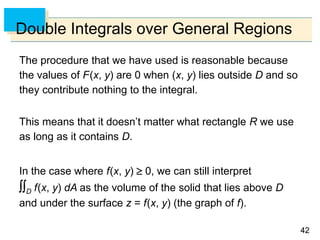
Double Integrals over General Regions
In order to evaluate D f(x, y) dA when D is a region of
type I, we choose a rectangle R = [a, b] [c, d] that
contains D, as in Figure 6, and we let F be the function
given by Equation 1; that is, F agrees with f on D and F is 0
outside D.
Figure 6](https://image.slidesharecdn.com/chatper15-191003195240/85/Chatper-15-46-320.jpg)


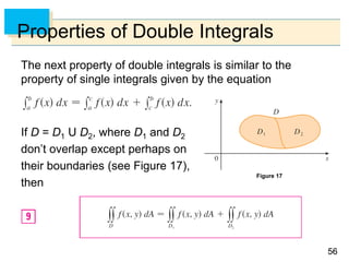
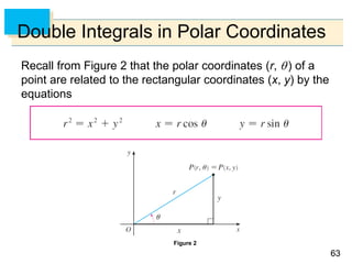
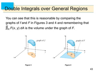
![6565
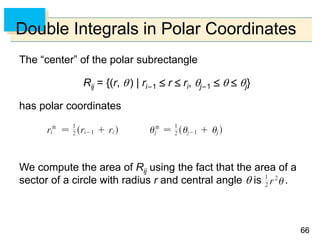
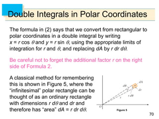
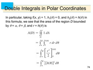
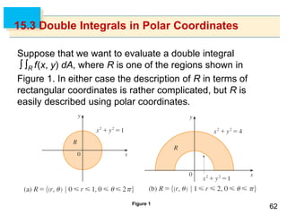
Double Integrals in Polar Coordinates
In order to compute the double integral R f(x, y) dA, where
R is a polar rectangle, we divide the interval [a, b] into m
subintervals [ri–1, ri] of equal width r = (b – a)/m and we
divide the interval [, ] into n subintervals [j–1, j] of
equal width = ( – )/n.
Then the circles r = ri and the
rays = j divide the polar
rectangle R into the small polar
rectangles Rij shown in Figure 4.
Figure 4
Dividing R into polar subrectangles](https://image.slidesharecdn.com/chatper15-191003195240/85/Chatper-15-65-320.jpg)