This document describes modeling and control of aircraft pitch dynamics. It presents: 1) The longitudinal equations of motion and state-space models of an aircraft's pitch. 2) Analysis of the open-loop system and design of an LQR controller for stable response. 3) Simulink modeling of the open-loop and closed-loop aircraft pitch systems.

1. MODERN CONTROL SYSTEM
Modern design of Aircraft Control System
By
Pourya Parsa
For
Professor: s.zeinolabedin Mousavi
TA: Reihaneh Amiri
Islamic Azad University Central
Tehran Branch
Islamic Azad University Central
Tehran Branch
Junuary 2017
modern control system project
Islamic Azad University Central
Tehran Branch

2. Physical setup and system equations
Aircraft pitch is governed by the longitudinal dynamics. In this
example we will design an autopilot that controls the pitch of an
aircraft.
The basic coordinate axes
and forces acting on an aircraft
are shown in the figure
modern control system project
Islamic Azad University Central
Tehran Branch

3. modern control system project
Islamic Azad University Central
Tehran Branch
We will assume that the aircraft is in steady-cruise at constant altitude
and velocity; thus, the thrust, drag, weight and lift forces balance
each other in the x- and y-directions. We will also assume that a
change in pitch angle will not change the speed of the aircraft under
any circumstance (unrealistic but simplifies the problem a bit). Under
these assumptions, the longitudinal equations of motion for the
aircraft can be written as follows

4. Transfer function and state-space models
modern control system project
These values are taken from the data from one of Boeing's
commercial aircraft
Islamic Azad University Central
Tehran Branch
1. Transfer function
The Laplace transform of the equations are shown
After few steps of algebra

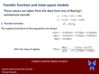
5. 2. State space
modern control system project
MATLAB representation
Continuous-time transfer function
Islamic Azad University Central
Tehran Branch
Continuous-time state-space model
s = tf('s');
P_pitch (1.151*s+0.1774)/(s^3+0.739*s^2+0.921*s
A = [-0.313 56.7 0; -0.0139 -0.426 0; 0 56.7 0];
B = [0.232; 0.0203; 0];
C = [0 0 1];
D = [0];
pitch_ss = ss(A,B,C,D)

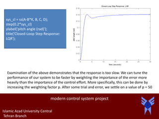
6. Controllability
modern control system project
Islamic Azad University Central
Tehran Branch
For the system to be completely state controllable, the controllability matrix
Since our controllability matrix is 3x3, the rank of the matrix must be 3.
The MATLAB command rank can give you the rank of this matrix
A = [-0.313 56.7 0; -0.0139 -0.426 0; 0 56.7 0];
B = [0.232; 0.0203; 0];
C = [0 0 1];
D = [0];
co = ctrb(A,B);
Controllability = rank(co)
Controllability =
3
Therefore, our system is completely state controllable since the controllability matrix
has rank 3.

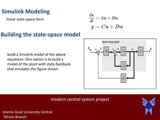
7. Control design via pole placement
modern control system project
Islamic Azad University Central
Tehran Branch
The schematic of a full-state feedback control system is shown below (with D = 0).
Based on the above, matrix A - BK
determines the closed-loop dynamics
of our system. Specfically, the roots of
the determinant of the matrix
[ sI - ( A - BK ) ] are the closed-loop
poles of the system. Since the
determinant of [ sI - ( A - BK ) ] is a
third-order polynomial, there are
three poles we can place and since
our system is completely state
controllable, we can place the poles
anywhere we like

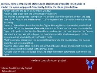
8. Linear quadratic regulation
modern control system project
Islamic Azad University Central
Tehran Branch
We will use a technique called the Linear Quadratic Regulator (LQR) method to generate
the "best" gain matrix K, without explicitly choosing to place the closed-loop poles in
particular locations. This type of control technique optimally balances the system error and
the control effort based on a cost that the designer specifies that defines the relative
importance of minimizing errors and minimimizing control effort. In the case of the
regulator problem, it is assumed that the reference is zero
p = 2;
Q = p*C'*C
R = 1;
[K] = lqr(A,B,Q,R)
Q =
0 0 0
0 0 0
0 0 2
K =
-0.5034 52.8645 1.4142

9. modern control system project
Islamic Azad University Central
Tehran Branch
sys_cl = ss(A-B*K, B, C, D);
step(0.2*sys_cl)
ylabel('pitch angle (rad)');
title('Closed-Loop Step Response:
LQR');
Examination of the above demonstrates that the response is too slow. We can tune the
performance of our system to be faster by weighting the importance of the error more
heavily than the importance of the control effort. More specifically, this can be done by
increasing the weighting factor p. After some trial and error, we settle on a value of p = 50

10. modern control system project
Islamic Azad University Central
Tehran Branch
Modify the code of your m-file as follows and then run at the command
line to produce the following step response.
p = 50;
Q = p*C'*C;
R = 1;
[K] = lqr(A,B,Q,R)
sys_cl = ss(A-B*K, B, C, D);
step(0.2*sys_cl) ylabel('pitch angle (rad)');
title('Closed-Loop Step Response: LQR');
K =
-0.6435 169.6950 7.0711

11. modern control system project
Islamic Azad University Central
Tehran Branch
Examination of demonstrates that the rise time, overshoot, and
settling time are satisfactory. However, there is a large steady-state
error. One way to correct this is by introducing a precompensator
.(Nbar) to scale the overall output

12. Simulink Modeling
modern control system project
Islamic Azad University Central
Tehran Branch
linear state-space form
Building the state-space model
build a Simulink model of the above
equations. One option is to build a
model of the plant with state-feedback
that emulates the figure shown

13. We will, rather, employ the State-Space block made available in Simulink to
model the open-loop plant. Specfically, follow the steps given below.
modern control system project
Islamic Azad University Central
Tehran Branch
*Open Simulink and open a new model window.
*Insert a Step block from the Simulink/Sources library.
*To provide a appropriate step input at t=0, double-click the Step block and set the Step
time to "0". Also set the Final value to "0.2" to represent the 0.2-radian reference we are
assuming.
*Insert a Demux block from the Simulink/Signal Routing library. Double-click on the block
and enter "3" for the Number of outputs; one output for each of the three state variables.
*Insert a Scope from the Simulink/Sinks library and connect the third output of the Demux
block to the scope. We will only plot the third state variable which corresponds to the
system's output which is the aircraft's pitch theta.
*Add Terminator blocks from the Simulink/Sinks library to the two signals of the Demux
block that we are not plotting.
*Insert a State-Space block from the Simulink/Continuous library and connect the input to
the Step block and the output to the Demux block.
*Double-click on the State-Space block and enter the system parameters as shown in the
figure

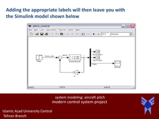
14. modern control system project
Islamic Azad University Central
Tehran Branch
In the figure the C matrix is entered as a 3x3
identity matrix using the eye command rather
than [0 0 1] as given in the original state-space
equations. The reason for this is because in
state-feedback control it is assumed that all of
the state variables are measured, not just the
output. If this is not the case, then an observer
needs to be designed to estimate any state
variables that are not measured. Refer to the
State-Space Methods for Controller Design.
When finished, the completed model should
appear in the next figure

15. modern control system project
Islamic Azad University Central
Tehran Branch

16. Generating the open-loop and closed-loop response
modern control system project
Islamic Azad University Central
Tehran Branch
Next generate the open-loop step response
by running the simulation

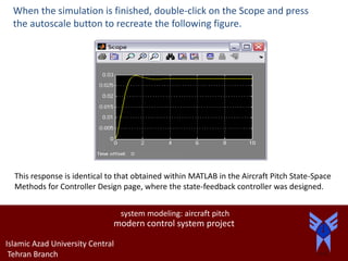
17. This response is unstable and identical
to that obtained within MATLAB in the
Aircraft Pitch System Analysis page. In
order to view a stable response, we
will now quickly add the state-
feedback control gain K designed in
the Aircraft Pitch: State-Space
Methods for Controller Design page.
Recall that this gain was designed
using the Linear Quadratic Regulator
method and resulted in a calculation
of K = [-0.6435 169.6950 7.0711].
modern control system project
Islamic Azad University Central
Tehran Branch

18. system modeling: aircraft pitch
modern control system project
Islamic Azad University Central
Tehran Branch
Adding the appropriate labels will then leave you with
the Simulink model shown below

19. When the simulation is finished, double-click on the Scope and press
the autoscale button to recreate the following figure.
system modeling: aircraft pitch
modern control system project
Islamic Azad University Central
Tehran Branch
This response is identical to that obtained within MATLAB in the Aircraft Pitch State-Space
Methods for Controller Design page, where the state-feedback controller was designed.