Download to read offline
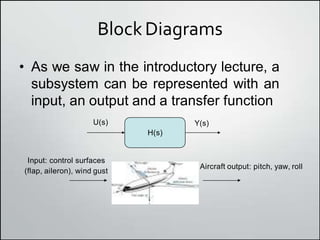

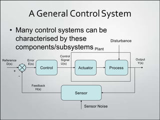
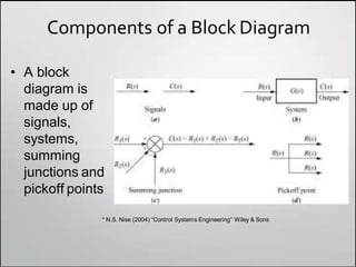
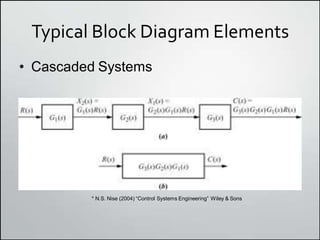
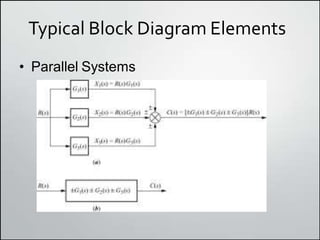
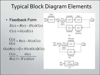
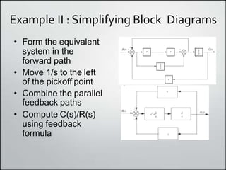
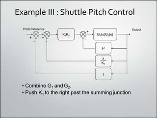
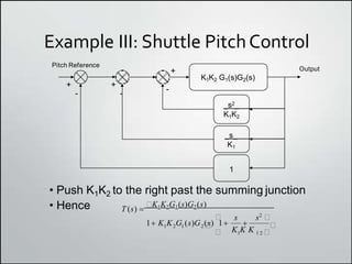
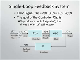
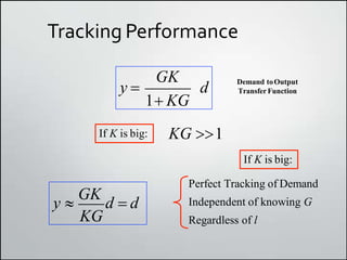
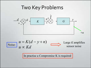

1. Block diagrams can be used to represent subsystems in a system using inputs, outputs, and transfer functions. Multiple subsystems can be combined using rules for cascaded, parallel, and feedback systems. 2. Simplifying block diagrams allows us to find the overall system transfer function by reducing the diagram to an equivalent form. Examples show how to simplify complex diagrams. 3. Feedback control is useful for rejecting disturbances and improving tracking performance, but large feedback gains can amplify sensor noise, so a compromise is needed.


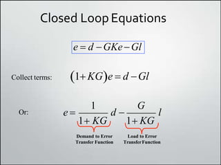
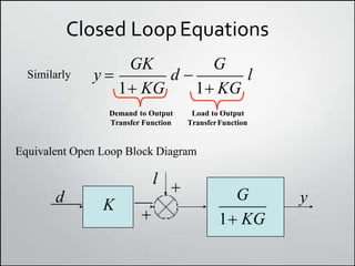
![Reduction of multiple subsystem [compatibility mode]](https://cdn.slidesharecdn.com/ss_thumbnails/reductionofmultiplesubsystemcompatibilitymode-110418075355-phpapp01-thumbnail.jpg?width=640&height=640&fit=bounds)