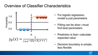
The document provides an overview of decision trees, including:
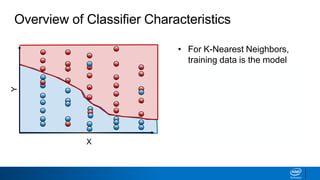
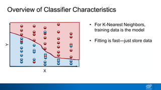
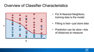
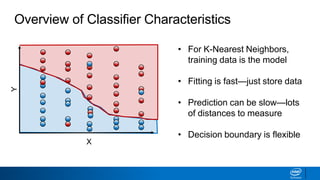
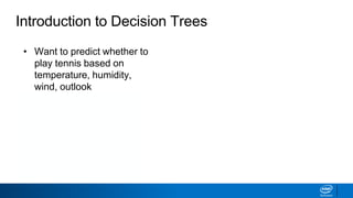
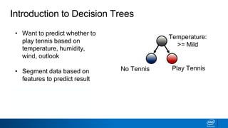
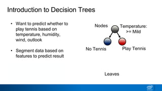
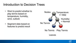
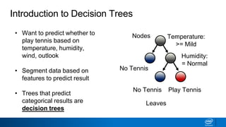
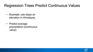
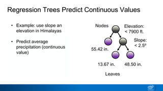
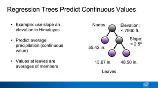
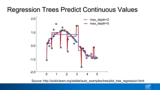
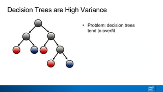
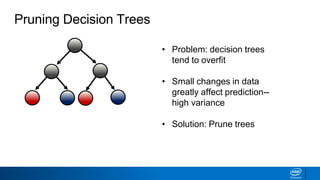
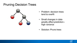
- Decision trees can be used for classification or regression problems by segmenting data based on features to predict categorical or continuous target values.
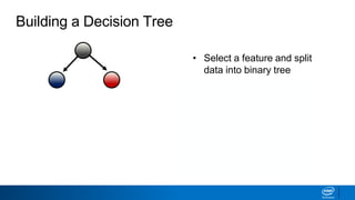
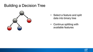
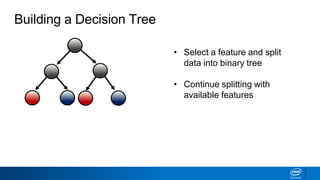
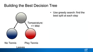
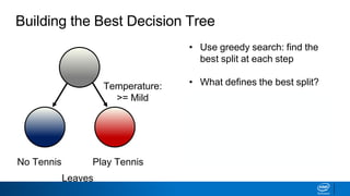
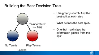
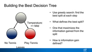
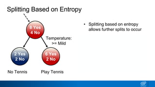
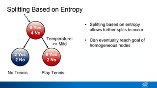
- The tree is built recursively by selecting the best feature to split the data on at each node, with the goal of maximizing information gain or minimizing entropy.
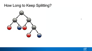
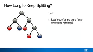
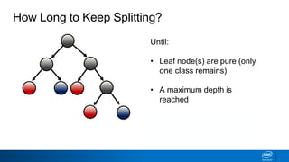
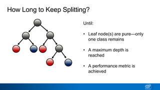
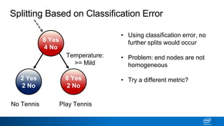
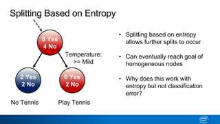
- Splits continue until nodes are pure or a stopping criteria like maximum depth is reached. Entropy works better than classification error as a splitting metric because it favors splits furthest from ambiguous 50/50 splits.


![Splitting Based on Classification Error
2 Yes
2 No
6 Yes
2 No
Play TennisNo Tennis
Temperature:
>= Mild
8 Yes
4 No 𝐸 𝑡 = 1 − max
𝑖
[𝑝 𝑖 𝑡 ]
Classification Error
Equation
Classification Error Before
1 − 8
12 = 0.3333](https://image.slidesharecdn.com/ml6-decisiontrees-190218095438/85/Ml6-decision-trees-34-320.jpg)
![Splitting Based on Classification Error
2 Yes
2 No
6 Yes
2 No
Play TennisNo Tennis
Temperature:
>= Mild
8 Yes
4 No 𝐸 𝑡 = 1 − max
𝑖
[𝑝 𝑖 𝑡 ]
Classification Error
Equation
Classification Error Before
1 − 8
12 = 0.3333](https://image.slidesharecdn.com/ml6-decisiontrees-190218095438/85/Ml6-decision-trees-35-320.jpg)
![Splitting Based on Classification Error
2 Yes
2 No
6 Yes
2 No
Play TennisNo Tennis
Temperature:
>= Mild
8 Yes
4 No 𝐸 𝑡 = 1 − max
𝑖
[𝑝 𝑖 𝑡 ]
Classification Error
Equation
Classification Error Left Side
1 − 2
4 = 0.5000
0.3333](https://image.slidesharecdn.com/ml6-decisiontrees-190218095438/85/Ml6-decision-trees-36-320.jpg)
![Splitting Based on Classification Error
2 Yes
2 No
6 Yes
2 No
Play TennisNo Tennis
Temperature:
>= Mild
8 Yes
4 No 𝐸 𝑡 = 1 − max
𝑖
[𝑝 𝑖 𝑡 ]
Classification Error
Equation
Classification Error Left Side
1 − 2
4 = 0.5000
0.3333
Information lost on
small # of data points](https://image.slidesharecdn.com/ml6-decisiontrees-190218095438/85/Ml6-decision-trees-37-320.jpg)
![Splitting Based on Classification Error
2 Yes
2 No
6 Yes
2 No
Play TennisNo Tennis
Temperature:
>= Mild
8 Yes
4 No 𝐸 𝑡 = 1 − max
𝑖
[𝑝 𝑖 𝑡 ]
Classification Error
Equation
Classification Error Right
Side
1 − 6
8 = 0.2500
0.3333
0.5000](https://image.slidesharecdn.com/ml6-decisiontrees-190218095438/85/Ml6-decision-trees-38-320.jpg)
![Splitting Based on Classification Error
2 Yes
2 No
6 Yes
2 No
Play TennisNo Tennis
Temperature:
>= Mild
8 Yes
4 No 𝐸 𝑡 = 1 − max
𝑖
[𝑝 𝑖 𝑡 ]
Classification Error
Equation
Classification Error Change
0.3333 − 4
12 ∗ 0.5000 − 8
12 ∗0.2500
= 0
0.3333
0.5000 0.2500](https://image.slidesharecdn.com/ml6-decisiontrees-190218095438/85/Ml6-decision-trees-39-320.jpg)
![Splitting Based on Classification Error
2 Yes
2 No
6 Yes
2 No
Play TennisNo Tennis
Temperature:
>= Mild
8 Yes
4 No 𝐸 𝑡 = 1 − max
𝑖
[𝑝 𝑖 𝑡 ]
Classification Error
Equation
Classification Error Change
0.3333
0.5000 0.2500
0.3333 − 4
12 ∗ 0.5000 − 8
12 ∗0.2500
= 0](https://image.slidesharecdn.com/ml6-decisiontrees-190218095438/85/Ml6-decision-trees-40-320.jpg)
![Splitting Based on Entropy
2 Yes
2 No
6 Yes
2 No
Play TennisNo Tennis
Temperature:
>= Mild
8 Yes
4 No
𝐻 𝑡 = −
𝑖=1
𝑛
𝑝 𝑖 𝑡 𝑙𝑜𝑔2[𝑝(𝑖|𝑡)]
Entropy Equation
Entropy Before
− 8
12 𝑙𝑜𝑔2(8
12) − 4
12 𝑙𝑜𝑔2(4
12) = 0.9183](https://image.slidesharecdn.com/ml6-decisiontrees-190218095438/85/Ml6-decision-trees-42-320.jpg)
![Splitting Based on Entropy
2 Yes
2 No
6 Yes
2 No
Play TennisNo Tennis
Temperature:
>= Mild
8 Yes
4 No
𝐻 𝑡 = −
𝑖=1
𝑛
𝑝 𝑖 𝑡 𝑙𝑜𝑔2[𝑝(𝑖|𝑡)]
Entropy Equation
Entropy Before
− 8
12 𝑙𝑜𝑔2(8
12) − 4
12 𝑙𝑜𝑔2(4
12) = 0.9183](https://image.slidesharecdn.com/ml6-decisiontrees-190218095438/85/Ml6-decision-trees-43-320.jpg)
![Splitting Based on Entropy
2 Yes
2 No
6 Yes
2 No
Play TennisNo Tennis
Temperature:
>= Mild
8 Yes
4 No
𝐻 𝑡 = −
𝑖=1
𝑛
𝑝 𝑖 𝑡 𝑙𝑜𝑔2[𝑝(𝑖|𝑡)]
Entropy Equation
Entropy Left Side
− 2
4 𝑙𝑜𝑔2(2
4) − 2
4 𝑙𝑜𝑔2(2
4) = 1.0000
0.9183](https://image.slidesharecdn.com/ml6-decisiontrees-190218095438/85/Ml6-decision-trees-44-320.jpg)
![Splitting Based on Entropy
2 Yes
2 No
6 Yes
2 No
Play TennisNo Tennis
Temperature:
>= Mild
8 Yes
4 No
𝐻 𝑡 = −
𝑖=1
𝑛
𝑝 𝑖 𝑡 𝑙𝑜𝑔2[𝑝(𝑖|𝑡)]
Entropy Equation
Entropy Right Side
− 6
8 𝑙𝑜𝑔2(6
8) − 2
8 𝑙𝑜𝑔2(2
8) = 0.8113
0.9183
1.0000](https://image.slidesharecdn.com/ml6-decisiontrees-190218095438/85/Ml6-decision-trees-45-320.jpg)
![Splitting Based on Entropy
2 Yes
2 No
6 Yes
2 No
Play TennisNo Tennis
Temperature:
>= Mild
8 Yes
4 No
𝐻 𝑡 = −
𝑖=1
𝑛
𝑝 𝑖 𝑡 𝑙𝑜𝑔2[𝑝(𝑖|𝑡)]
Entropy Equation
Entropy Change
0.9183 − 4
12 ∗ 1.0000 − 8
12 ∗0.8113
= 0.0441
0.9183
1.0000 0.8113](https://image.slidesharecdn.com/ml6-decisiontrees-190218095438/85/Ml6-decision-trees-46-320.jpg)
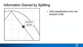
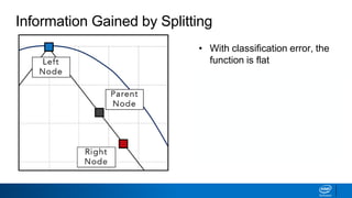
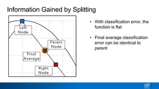
![• Classification error is a flat
function with maximum at
center
• Center represents
ambiguity—50/50 split
• Splitting metrics favor results
that are furthest away from
the center
Classification Error vs Entropy
0.0 0.5
Purity
1.0
Classification
Error
𝐸 𝑡 = 1 − max
𝑖
[𝑝 𝑖 𝑡 ]
Error](https://image.slidesharecdn.com/ml6-decisiontrees-190218095438/85/Ml6-decision-trees-50-320.jpg)
![• Classification error is a flat
function with maximum at
center
• Center represents
ambiguity—50/50 split
• Splitting metrics favor results
that are furthest away from
the center
Classification Error vs Entropy
0.0 0.5
Purity
1.0
Classification
Error
𝐸 𝑡 = 1 − max
𝑖
[𝑝 𝑖 𝑡 ]
Error](https://image.slidesharecdn.com/ml6-decisiontrees-190218095438/85/Ml6-decision-trees-51-320.jpg)
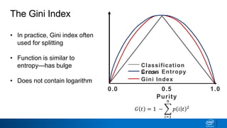
![0.0 0.5
Purity
1.0
Classification
Error
• Classification error is a flat
function with maximum at
center
• Center represents
ambiguity—50/50 split
• Splitting metrics favor results
that are furthest away from
the center
𝐸 𝑡 = 1 − max
𝑖
[𝑝 𝑖 𝑡 ]
Classification Error vs Entropy
Error](https://image.slidesharecdn.com/ml6-decisiontrees-190218095438/85/Ml6-decision-trees-52-320.jpg)
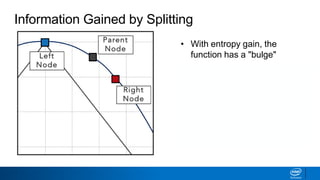
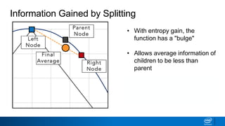
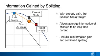
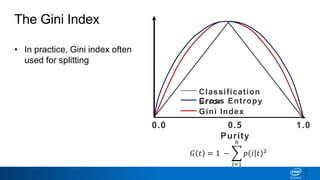
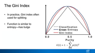
![Classification Error vs Entropy
• Entropy has the same
maximum but is curved
• Curvature allows splitting to
continue until nodes are pure
• How does this work?
0.0 0.5
Purity
1.0
Classification
ErrorCross Entropy
𝐻 𝑡 = −
𝑖=1
𝑛
𝑝 𝑖 𝑡 𝑙𝑜𝑔2[𝑝(𝑖|𝑡)]
Error/Entropy](https://image.slidesharecdn.com/ml6-decisiontrees-190218095438/85/Ml6-decision-trees-53-320.jpg)
![Classification Error vs Entropy
• Entropy has the same
maximum but is curved
• Curvature allows splitting to
continue until nodes are pure
• How does this work?
0.0 0.5
Purity
1.0
Classification
ErrorCross Entropy
𝐻 𝑡 = −
𝑖=1
𝑛
𝑝 𝑖 𝑡 𝑙𝑜𝑔2[𝑝(𝑖|𝑡)]
Error/Entropy](https://image.slidesharecdn.com/ml6-decisiontrees-190218095438/85/Ml6-decision-trees-54-320.jpg)
![0.0 0.5
Purity
1.0
Classification
ErrorCross Entropy
Classification Error vs Entropy
• Entropy has the same
maximum but is curved
• Curvature allows splitting to
continue until nodes are pure
• How does this work?
𝐻 𝑡 = −
𝑖=1
𝑛
𝑝 𝑖 𝑡 𝑙𝑜𝑔2[𝑝(𝑖|𝑡)]
Error/Entropy](https://image.slidesharecdn.com/ml6-decisiontrees-190218095438/85/Ml6-decision-trees-55-320.jpg)

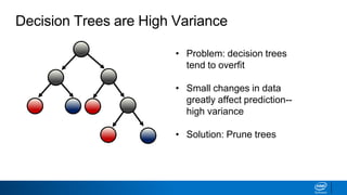
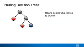
![• How to decide what leaves
to prune?
• Solution: prune based on
classification error threshold
Pruning Decision Trees
𝐸 𝑡 = 1 − max
𝑖
[𝑝 𝑖 𝑡 ]](https://image.slidesharecdn.com/ml6-decisiontrees-190218095438/85/Ml6-decision-trees-72-320.jpg)