Download as PDF, PPTX

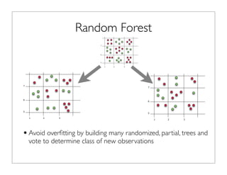
![ClassificationTrees
•Consider a supervised learning problem with a simple data set with
two classes and the data has two features x in [1,4] and y in [5,8].
•We can build a classification tree to predict classes of new
observations
1 2 3
6
5
7](https://image.slidesharecdn.com/janvitekdistributedrandomforest5-2-2013-130504133205-phpapp02/85/Jan-vitek-distributedrandomforest_5-2-2013-4-320.jpg)
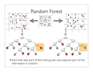
![ClassificationTrees
•Consider a supervised learning problem with a simple data set with
two classes and the data has two features x in [1,4] and y in [5,8].
•We can build a classification tree to predict classes of new
observations
1 2 3
6
5
7
>3
>6
>7
>2
>6
>7
2.6
6.5
>6
>7
5.5](https://image.slidesharecdn.com/janvitekdistributedrandomforest5-2-2013-130504133205-phpapp02/85/Jan-vitek-distributedrandomforest_5-2-2013-5-320.jpg)
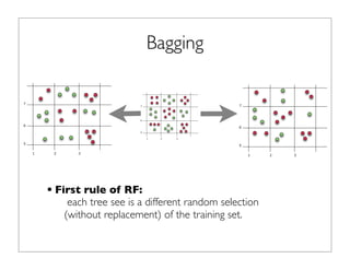

![Sample tree
• // Column constants
int COLSEPALLEN = 0;
int COLSEPALWID = 1;
int COLPETALLEN = 2;
int COLPETALWID = 3;
int classify(float fs[]) {
if( fs[COLPETALWID] <= 0.800000 )
return Iris-setosa;
else
if( fs[COLPETALLEN] <= 4.750000 )
if( fs[COLPETALWID] <= 1.650000 )
return Iris-versicolor;
else
return Iris-virginica;
else
if( fs[COLSEPALLEN] <= 6.050000 )
if( fs[COLPETALWID] <= 1.650000 )
return Iris-versicolor;
else
return Iris-virginica;
else
return Iris-virginica;
}](https://image.slidesharecdn.com/janvitekdistributedrandomforest5-2-2013-130504133205-phpapp02/85/Jan-vitek-distributedrandomforest_5-2-2013-15-320.jpg)
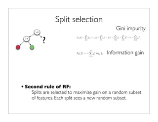
![Evaluating splits
•The implementation of entropy based split is now simple
Split ltSplit(int col, Data d, int[] dist, Random rand) {
final int[] distL = new int[d.classes()], distR = dist.clone();
final double upperBoundReduction = upperBoundReduction(d.classes());
double maxReduction = -1; int bestSplit = -1;
for (int i = 0; i < columnDists[col].length - 1; ++i) {
for (int j = 0; j < distL.length; ++j) {
double v = columnDists[col][i][j]; distL[j] += v; distR[j] -= v;
}
int totL = 0, totR = 0;
for (int e: distL) totL += e;
for (int e: distR) totR += e;
double eL = 0, eR = 0;
for (int e: distL) eL += gain(e,totL);
for (int e: distR) eR += gain(e,totR);
double eReduction = upperBoundReduction-( (eL*totL + eR*totR) / (totL+totR) );
if (eReduction > maxReduction) { bestSplit = i; maxReduction = eReduction; }
}
return Split.split(col,bestSplit,maxReduction);](https://image.slidesharecdn.com/janvitekdistributedrandomforest5-2-2013-130504133205-phpapp02/85/Jan-vitek-distributedrandomforest_5-2-2013-25-320.jpg)
![Parallelizing tree building
•Trees are built in parallel with the Fork/Join framework
Statistic left = getStatistic(0,data, seed + LTSSINIT);
Statistic rite = getStatistic(1,data, seed + RTSSINIT);
int c = split.column, s = split.split;
SplitNode nd = new SplitNode(c, s,…);
data.filter(nd,res,left,rite);
FJBuild fj0 = null, fj1 = null;
Split ls = left.split(res[0], depth >= maxdepth);
Split rs = rite.split(res[1], depth >= maxdepth);
if (ls.isLeafNode()) nd.l = new LeafNode(...);
else fj0 = new FJBuild(ls,res[0],depth+1, seed + LTSINIT);
if (rs.isLeafNode()) nd.r = new LeafNode(...);
else fj1 = new FJBuild(rs,res[1],depth+1, seed - RTSINIT);
if (data.rows() > ROWSFORKTRESHOLD)…
fj0.fork();
nd.r = fj1.compute();
nd.l = fj0.join();](https://image.slidesharecdn.com/janvitekdistributedrandomforest5-2-2013-130504133205-phpapp02/85/Jan-vitek-distributedrandomforest_5-2-2013-26-320.jpg)
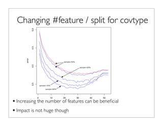
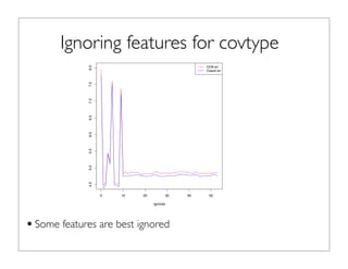


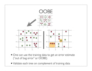
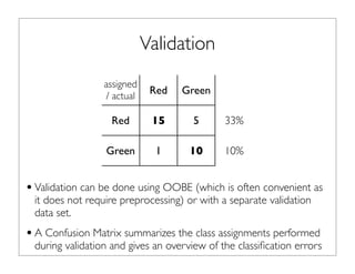
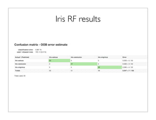
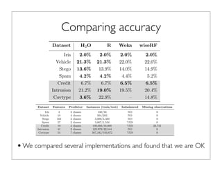
The document outlines the development and implementation of distributed random forests, detailing the advantages of using this approach for classification tasks in machine learning. It covers key concepts such as bagging, out-of-bag error estimation, and the impact of varying sampling rates and feature selection on model accuracy. The discussion includes practical examples using datasets like Iris and Covtype, as well as performance comparisons of various tools.