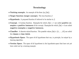
Download to read offline
![Sample Applications
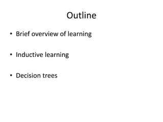
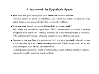
• Web search
• Computational biology
• Finance
• E-commerce
• Space exploration
• Robotics
• Information extraction
• Social networks
• Debugging
• [Your favorite area]](https://image.slidesharecdn.com/jdavis-indlearn2-240220113611-45701426/85/introduction-to-machine-learning-3c-pptx-6-320.jpg)
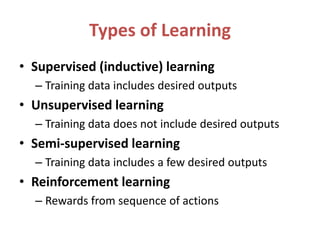

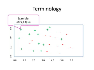
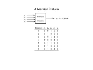
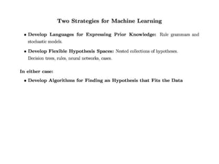


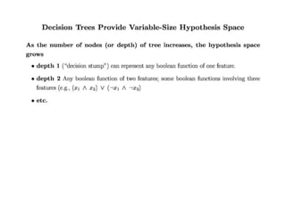
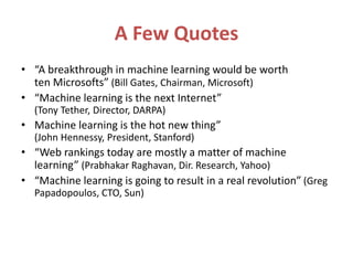
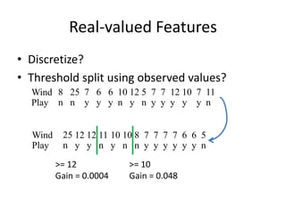
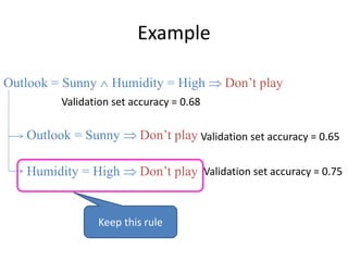
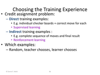
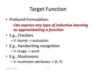
![What is the
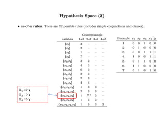
Simplest Tree?
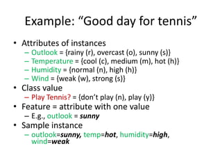
Day Outlook Temp Humid Wind Play?
d1 s h h w n
d2 s h h s n
d3 o h h w y
d4 r m h w y
d5 r c n w y
d6 r c n s n
d7 o c n s y
d8 s m h w n
d9 s c n w y
d10 r m n w y
d11 s m n s y
d12 o m h s y
d13 o h n w y
d14 r m h s n
How good?
[9+, 5-]
Majority class:
correct on 9 examples
incorrect on 5 examples](https://image.slidesharecdn.com/jdavis-indlearn2-240220113611-45701426/85/introduction-to-machine-learning-3c-pptx-46-320.jpg)
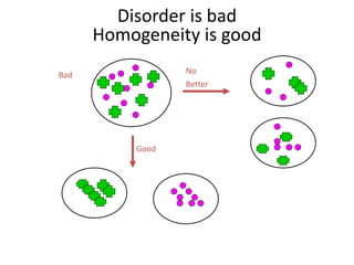
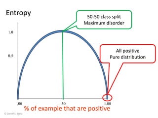
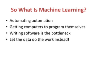
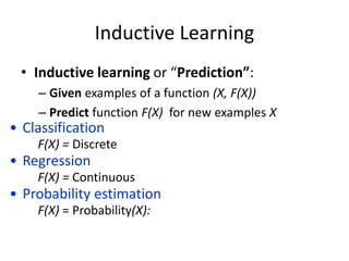
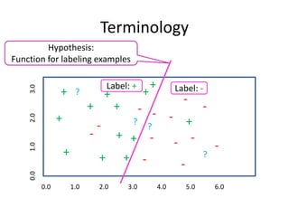
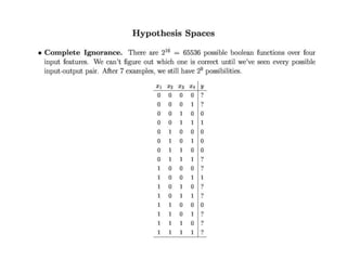
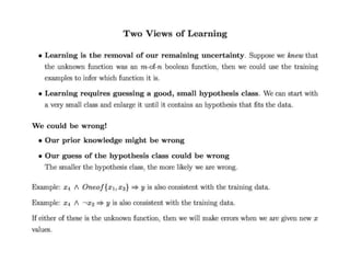
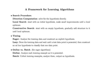
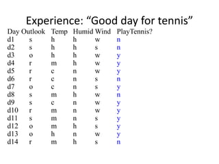
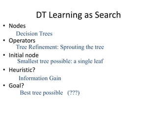
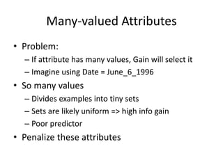
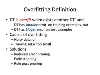
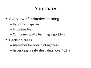
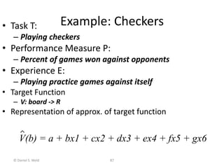
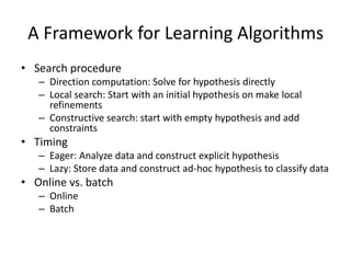
![Entropy (disorder) is bad
Homogeneity is good
• Let S be a set of examples
• Entropy(S) = -P log2(P) - N log2(N)
– P is proportion of pos example
– N is proportion of neg examples
– 0 log 0 == 0
• Example: S has 9 pos and 5 neg
Entropy([9+, 5-]) = -(9/14) log2(9/14) -
(5/14)log2(5/14)
= 0.940](https://image.slidesharecdn.com/jdavis-indlearn2-240220113611-45701426/85/introduction-to-machine-learning-3c-pptx-50-320.jpg)
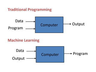
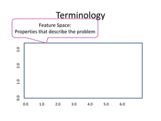
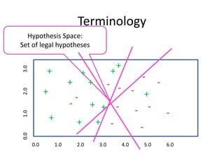
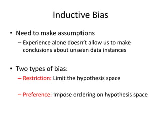
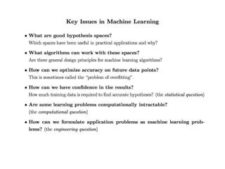
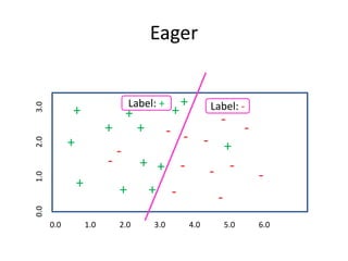
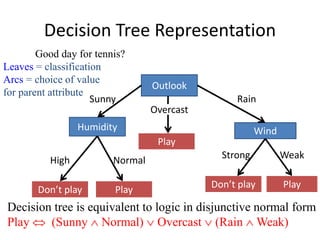
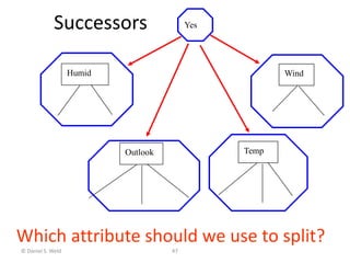
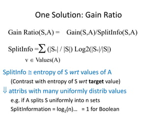
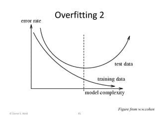
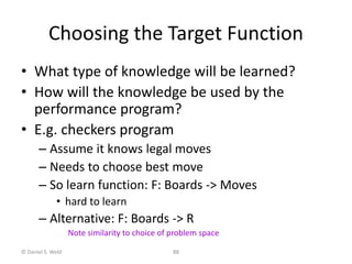
![Day Wind Tennis?
d1 weak n
d2 s n
d3 weak yes
d4 weak yes
d5 weak yes
d6 s n
d7 s yes
d8 weak n
d9 weak yes
d10 weak yes
d11 s yes
d12 s yes
d13 weak yes
d14 s n
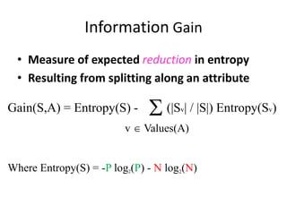
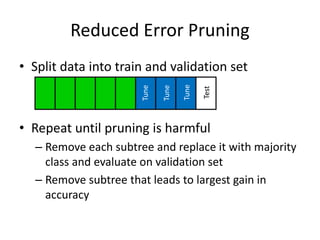
Gain of Splitting on Wind
Values(wind)=weak, strong
S = [9+, 5-]
Gain(S, wind)
= Entropy(S) - (|Sv| / |S|) Entropy(Sv)
= Entropy(S) - 8/14 Entropy(Sweak)
- 6/14 Entropy(Ss)
= 0.940 - (8/14) 0.811 - (6/14) 1.00
= .048
v {weak, s}
Sweak = [6+, 2-]
Ss = [3+, 3-]](https://image.slidesharecdn.com/jdavis-indlearn2-240220113611-45701426/85/introduction-to-machine-learning-3c-pptx-52-320.jpg)
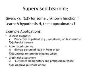
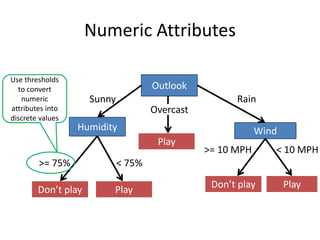
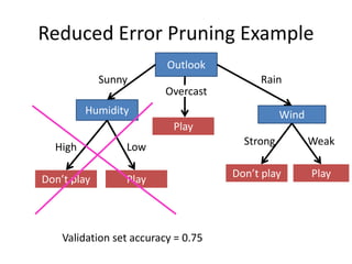
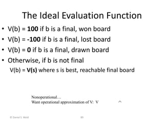
![Resulting Tree
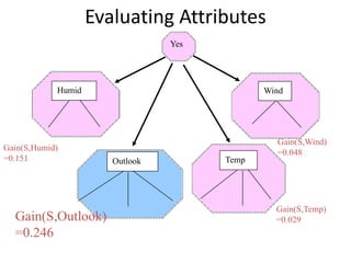
Outlook
Sunny Rain
Overcast
Good day for tennis?
Don’t Play
[2+, 3-] Play
[4+]
Don’t Play
[3+, 2-]](https://image.slidesharecdn.com/jdavis-indlearn2-240220113611-45701426/85/introduction-to-machine-learning-3c-pptx-55-320.jpg)
![One Step Later
Outlook
Humidity
Sunny Rain
Overcast
High
Normal
Play
[2+]
Play
[4+]
Don’t play
[3-]
Good day for tennis?
Don’t Play
[2+, 3-]](https://image.slidesharecdn.com/jdavis-indlearn2-240220113611-45701426/85/introduction-to-machine-learning-3c-pptx-57-320.jpg)
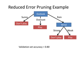
![One Step Later: Final Tree
Outlook
Humidity
Sunny Rain
Overcast
High
Normal
Play
[2+]
Play
[4+]
Don’t play
[3-]
Good day for tennis?
Wind
Weak
Strong
Play
[3+]
Don’t play
[2-]](https://image.slidesharecdn.com/jdavis-indlearn2-240220113611-45701426/85/introduction-to-machine-learning-3c-pptx-59-320.jpg)
![Missing Data 2
• 75% h and 25% n
• Use in gain calculations
• Further subdivide if other missing attributes
• Same approach to classify test ex with missing attr
– Classification is most probable classification
– Summing over leaves where it got divided
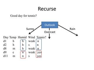
Day Temp Humid Wind Tennis?
d1 h h weak n
d2 h h s n
d8 m h weak n
d9 c ? weak yes
d11 m n s yes
[0.75+, 3-]
[1.25+, 0-]](https://image.slidesharecdn.com/jdavis-indlearn2-240220113611-45701426/85/introduction-to-machine-learning-3c-pptx-62-320.jpg)

![Gain of Split
on Humidity
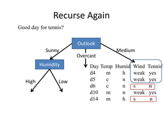
Day Outlook Temp Humid Wind Play?
d1 s h h w n
d2 s h h s n
d3 o h h w y
d4 r m h w y
d5 r c n w y
d6 r c n s n
d7 o c n s y
d8 s m h w n
d9 s c n w y
d10 r m n w y
d11 s m n s y
d12 o m h s y
d13 o h n w y
d14 r m h s n
Entropy([9+,5-]) = 0.940
Entropy([4+,3-]) = 0.985
Entropy([6+,-1]) = 0.592
Gain = 0.940- 0.985/2 - 0.592/2= 0.151](https://image.slidesharecdn.com/jdavis-indlearn2-240220113611-45701426/85/introduction-to-machine-learning-3c-pptx-82-320.jpg)


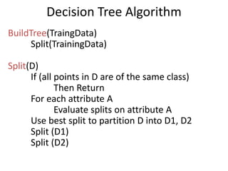
Machine learning allows computers to learn from data without being explicitly programmed. The document discusses supervised inductive learning where the goal is to predict an output value given an input. Decision trees are a popular method that represent learned functions as tree structures. The document provides an example of learning a decision tree to predict whether it is a good day for tennis given attributes like temperature and wind. It describes how decision trees are learned by splitting the training data on attributes that provide the most information gain at each step, resulting in a tree that can classify new examples.