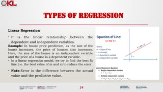
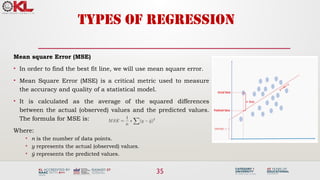
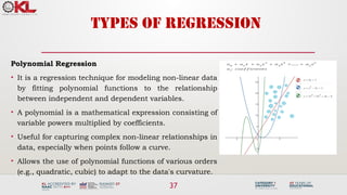
Download to read offline
![5
VARIANCE
• Variance in machine learning refers to the model's sensitivity to fluctuations or
noise in the data.
• High Variance: A high-variance model takes into account not only the underlying
patterns but also the noise in the training data. This means it learns too much
from the training data, leading to issues when making predictions on new (testing)
data.
• Mathematical Representation: The variance error in the model can be
mathematically expressed as:
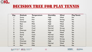
Variancef(x)) = E[X^2] - E[X]^2](https://image.slidesharecdn.com/3-240810113905-c6ec7e78/85/3-Tree-Models-in-machine-learning-5-320.jpg)
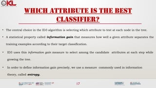
![20
Which attribute is the best
classifier?
A1=?
True False
[21+, 5-] [8+, 30-]
[29+,35-]
A2=?
True False
[18+, 33-] [11+, 2-]
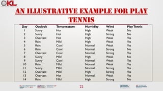
[29+,35-]](https://image.slidesharecdn.com/3-240810113905-c6ec7e78/85/3-Tree-Models-in-machine-learning-20-320.jpg)
![21
Which attribute is the best
classifier?
𝐸𝑛𝑡𝑟𝑜𝑝𝑦 ([ 29+ , 35 −] )=−
29
64
log2
29
64
−
35
64
log 2
35
64
=0.99
•
0.12
•
0.27
• A1 provides greater information gain than A2, So A1 is a better classifier than A2.](https://image.slidesharecdn.com/3-240810113905-c6ec7e78/85/3-Tree-Models-in-machine-learning-21-320.jpg)
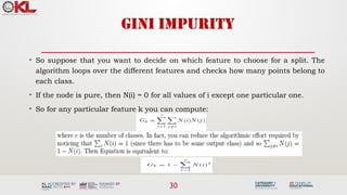
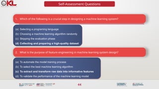
![Selecting next attribute
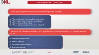
• Entropy([9+,5-] = – (9/14) log2(9/14) – (5/14) log2(5/14) = 0.940
Sunny Rain
S=[9+,5-]
E=0.940
[2+, 3-]
E=0.971
[3+, 2-]
E=0.971
Gain(S, Outlook) = 0.940-(5/14)*0.971 -(4/14)*0.0
-(5/14)*0.0971
= 0.247
Overcast
[4+, 0]
E=0.0
Hot Cold
S=[9+,5-]
E=0.940
[2+, 2-]
E=1.0
[3+, 1-]
E=0.811
Gain(S, Temp) = 0.940-(4/14)*1.0 - (6/14)*0.911
- (4/14)*0.811
= 0.029
Mild
[4+, 2-]
E= 0.911
Outlook Temperature](https://image.slidesharecdn.com/3-240810113905-c6ec7e78/85/3-Tree-Models-in-machine-learning-23-320.jpg)
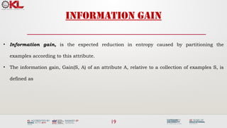
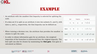
![24
Selecting next attribute
Humidity
High Normal
[3+, 4-] [6+, 1-]
S=[9+,5-]
E=0.940
Gain(S, Humidity) = 0.940-(7/14)*0.985-(7/14)*0.592
= 0.151
E=0.592
Wind
Weak Strong
[6+, 2-] [3+, 3-]
S=[9+,5-]
E=0.940
Gain(S, Wind) = 0.940-(8/14)*0.811-(6/14)*1.0
= 0.048
E=0.985](https://image.slidesharecdn.com/3-240810113905-c6ec7e78/85/3-Tree-Models-in-machine-learning-24-320.jpg)
![25
Best attribute-outlook
• The information gain values for the 4 attributes are:
• Gain(S, Outlook) = 0.247
• Gain(S, Temp) = 0.029
• Gain(S, Humidity) = 0.151
• Gain(S, Wind) = 0.048
Sunny Rain
[2+, 3-]
S=[9+,5-]
S={D1,D2,…,D14}
Overcast
[3+, 2-]
Srain={D4,D5,D6,D10,D14}
[4+, 0]
Sovercast={D3,D7,D12,D13}
Which attribute should be tested here?
Outlook
Yes
? ?
Ssunny={D1,D2,D8,D9,D11}](https://image.slidesharecdn.com/3-240810113905-c6ec7e78/85/3-Tree-Models-in-machine-learning-25-320.jpg)
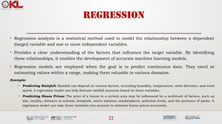
![27
ID3-result
Outlook
Sunny Overcast Rain
Humidity
[D3,D7,D12,D13]
Strong Weak
Yes
Yes
[D8,D9,D11]
No
[D6,D14]
Yes
[D4,D5,D10]
No
[D1,D2]
High Normal
Wind](https://image.slidesharecdn.com/3-240810113905-c6ec7e78/85/3-Tree-Models-in-machine-learning-27-320.jpg)

The document discusses machine learning tree models, focusing on decision trees and their applications in classification and regression tasks. It covers key concepts like bias-variance tradeoff, the ID3 algorithm for constructing decision trees, and regression analysis, along with common methods like linear regression and metrics such as mean square error. The session aims to equip learners with the understanding and skills to apply decision tree learning techniques to real-world datasets.