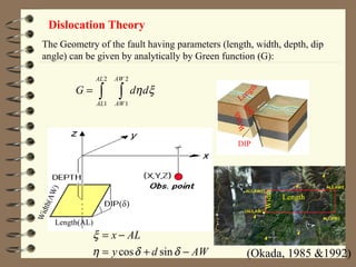
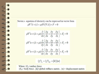
Method of Modelling
Kutubuddin ANSARI
kutubuddin.ansari@ikc.edu.tr
GNSS Surveying, GE 205
Lecture 12, May 22, 2015
The Geometry of the fault having parameters (length, width, depth, dip
angle) can be given by analytically by Green function (G):
2 2
1 1
AL AW
AL AW
G d dη ξ= ∫ ∫
(Okada, 1985 &1992)
Length
Width
DIP
Slip
Length(AL)
Width(AW)
Length
Width
cos sin
x AL
y d AW
ξ
η δ δ
= −
= + −
(δ)
Dislocation Theory
(P. Cervelli et. al 2001)
S is Slip For Oblique Slip
S= s.cosα + s.sinα
d= sG(m)
Relationship between dislocation field (d) and the fault
geometry G(m)
Since the ruptured area is not a perfect finite rectangular
and it contains error the Cervelli equation becomes
Forward Modelling Approach
d= sG(m)+
d-sG(m)
0
ˆ ˆ ˆd= sG(m)
if
ε
ε
ε
=
→
where
m=initial model parameter
ˆ mod
ˆ mod
ˆ mod
s slip
error
S Net slip
d elled dislocaton field
s el slip
m el parameter
rake of the netslip on the fault plane
ε
α
=
=
=
=
=
=
=For Oblique Slip
S= s.cosα + s.sinα
Coulomb Software
Coulomb software is based on the Boundary
Element Method (BEM). The inputs given to
Coulomb are estimates of length, width, dip
angle, strike slip and dip slip of the modelled
fault plane as well as the co-ordinates of the
trace of the fault plane.
(Toda et al., 2010)
Coulomb Input File (Toda et al., 2010)
The relation between displacement field and the source geometry can be
expressed by the following equation:
( )
( )
d G m
d sG m
α
=
Where d= displacement vector
m=source geometry (dislocation, length, width, depth, strike, dip)
s=slip
(P. Cervelli et al., 2001)
Inverse Modelling
If we have observed data d1
, d2
, …dn
and the Green function of each
observation data are G1
, G2
, …Gn
respectively, Then-
1 11 12 1 1
2 21 22 2 2
1 2
.........
.........
. . .
. . .
. . .
.........
m
m
n n n nm m
d G G G m
d G G G m
d G G G m
    
    
    
    
=    
    
    
    
        
1
1 11 12 1 1
2 21 22 2 2
1 2
.........
.........
. . .
. . .
. . .
.........
m
m
m n n nm n
m G G G d
m G G G d
m G G G d
−
     
     
     
     
=     
     
     
     
          
Least square approach
Cartesian Co-ordinate system (x,y,z) the half space occupied
region z<0 if fault is located at (0,0,-d) the point force
distribution can be given in following form .
Finite Element Method
μ, λ are lames constants
Thrust faults :-
F1 and F2 will be horizontal and F3 will be vertical.
Normal faults:-
F2 and F3 will be horizontal and F1 will be vertical
Strike-slip faults:-
F1 and F3 will be horizontal and F2 will be vertical
ANSYS (Brick 8 node 185) element, White concentrated area is
showing finite rectangular fault
Where Fi is acting force and ui and vi displacements of
points and ki
j are Stifness constants
At location of fault points
Method of fault modelling

Method of fault modelling

  • 1.
    Method of Modelling KutubuddinANSARI kutubuddin.ansari@ikc.edu.tr GNSS Surveying, GE 205 Lecture 12, May 22, 2015
  • 2.
    The Geometry ofthe fault having parameters (length, width, depth, dip angle) can be given by analytically by Green function (G): 2 2 1 1 AL AW AL AW G d dη ξ= ∫ ∫ (Okada, 1985 &1992) Length Width DIP Slip Length(AL) Width(AW) Length Width cos sin x AL y d AW ξ η δ δ = − = + − (δ) Dislocation Theory
  • 3.
    (P. Cervelli et.al 2001) S is Slip For Oblique Slip S= s.cosα + s.sinα d= sG(m) Relationship between dislocation field (d) and the fault geometry G(m)
  • 4.
    Since the rupturedarea is not a perfect finite rectangular and it contains error the Cervelli equation becomes Forward Modelling Approach d= sG(m)+ d-sG(m) 0 ˆ ˆ ˆd= sG(m) if ε ε ε = → where m=initial model parameter ˆ mod ˆ mod ˆ mod s slip error S Net slip d elled dislocaton field s el slip m el parameter rake of the netslip on the fault plane ε α = = = = = = =For Oblique Slip S= s.cosα + s.sinα
  • 5.
    Coulomb Software Coulomb softwareis based on the Boundary Element Method (BEM). The inputs given to Coulomb are estimates of length, width, dip angle, strike slip and dip slip of the modelled fault plane as well as the co-ordinates of the trace of the fault plane. (Toda et al., 2010)
  • 6.
    Coulomb Input File(Toda et al., 2010)
  • 7.
    Coulomb Input File(Toda et al., 2010)
  • 8.
    The relation betweendisplacement field and the source geometry can be expressed by the following equation: ( ) ( ) d G m d sG m α = Where d= displacement vector m=source geometry (dislocation, length, width, depth, strike, dip) s=slip (P. Cervelli et al., 2001) Inverse Modelling
  • 9.
    If we haveobserved data d1 , d2 , …dn and the Green function of each observation data are G1 , G2 , …Gn respectively, Then- 1 11 12 1 1 2 21 22 2 2 1 2 ......... ......... . . . . . . . . . ......... m m n n n nm m d G G G m d G G G m d G G G m                     =                             1 1 11 12 1 1 2 21 22 2 2 1 2 ......... ......... . . . . . . . . . ......... m m m n n nm n m G G G d m G G G d m G G G d −                         =                                   Least square approach
  • 10.
    Cartesian Co-ordinate system(x,y,z) the half space occupied region z<0 if fault is located at (0,0,-d) the point force distribution can be given in following form . Finite Element Method μ, λ are lames constants
  • 11.
    Thrust faults :- F1and F2 will be horizontal and F3 will be vertical. Normal faults:- F2 and F3 will be horizontal and F1 will be vertical Strike-slip faults:- F1 and F3 will be horizontal and F2 will be vertical
  • 13.
    ANSYS (Brick 8node 185) element, White concentrated area is showing finite rectangular fault
  • 14.
    Where Fi isacting force and ui and vi displacements of points and ki j are Stifness constants
  • 15.
    At location offault points