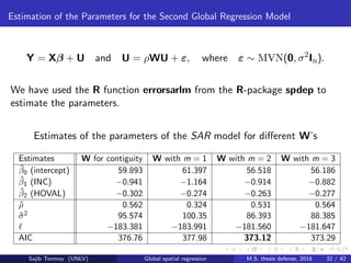
SlideShare a Scribd company logo
1 of 42
Download to read offline
Estimation of the parameters
in a spatial regressive-autoregressive model
using Ord’s eigenvalue method
Sajib Tonmoy
Department of Mathematical Sciences
University of Nevada, Las Vegas
M.S. thesis defense, 2018
Sajib Tonmoy (UNLV) Global spatial regression M.S. thesis defense, 2018 1 / 42
Outline
Ord (1975) considered spatial regressive-autoregressive models to describe
the interaction between location and a response variable in the presence of
several covariates (predictors).
He also developed a practical estimation method of the parameters of this
regression model.
In this thesis, we reviewed his estimation method and implemented it in
the statistical package R.
Sajib Tonmoy (UNLV) Global spatial regression M.S. thesis defense, 2018 2 / 42
The Models of Whittle, Bartlett, and Besag
For i = 1, . . . , n, suppose Yi is a response variable at location i. To describe the spatial
interaction between locations for the response variable, Whittle (1954) considered the
following autoregressive model:
Yi = α + ρ
j∈J(i)
wij Yj + εi (i = 1, . . . , n). (1)
Here,
ρ and α are parameters;
the εi ’s (i = 1, . . . , n) are random disturbance terms which are uncorrelated, have
equal variances, and zero means;
the wij ’s are non-negative weights (with wii = 0) that represent the “degree of
interactions” of each location i with the set of neighboring locations
J(i) = {i1, i2, . . . , imi }.
Remark
Here, J(i) may include all locations except location i. Note that,
n
i=1
J(i) ⊆ {1, 2, . . . , n}.
Sajib Tonmoy (UNLV) Global spatial regression M.S. thesis defense, 2018 3 / 42
The Models of Whittle, Bartlett, and Besag (cont.)
Bartlett (1966, 1971) and Besag (1972) considered the following conditional model:
E[Yi | Yj = yj , j ∈ J(i) ] = α + ρ
k∈J(i)
wik yk (i = 1, . . . , n). (2)
The following lemma shows the relationship between models (1) and (2):
Lemma
(a) If equations (1) and (2) hold, then
E[εi | Yj = yj , j ∈ J(i)] = 0 (i = 1, . . . , n). (3)
(b) If equations (1) and (3) hold, then equation (2) holds as well.
Sajib Tonmoy (UNLV) Global spatial regression M.S. thesis defense, 2018 4 / 42
Ord’s Global Regression Models
The first global spatial regression model Ord (1975) considered is
Y = Xβ + ρWY + ε, where ε ∼ MVN(0, σ2In).
Here,
X is an n × p design matrix;
β is a p × 1 vector of (unknown) coefficients;
W is an n × n weight matrix, whose (i, j)-th element is wij ;
Y = (y1, . . . , yn) is an n × 1 vector of response variables;
ε = (ε1, . . . , εn) is an n × 1 vector of random disturbance terms; and
ρ is an unknown parameter.
Sajib Tonmoy (UNLV) Global spatial regression M.S. thesis defense, 2018 5 / 42
Ord’s Global Regression Models (cont.)
The second global spatial regression model Ord (1975) considered is
Y = Xβ + U and U = ρWU + ε, where ε ∼ MVN(0, σ2In).
Here,
X is an n × p design matrix;
β is a p × 1 vector of (unknown) coefficients;
W is an n × n weight matrix, whose (i, j)-th element is wij ;
Y = (y1, . . . , yn) is an n × 1 vector of response variables;
ε = (ε1, . . . , εn) is an n × 1 vector of random disturbance terms;
U = (u1, . . . , un) is an n × 1 vector of disturbance terms; and
ρ is an unknown parameter.
Sajib Tonmoy (UNLV) Global spatial regression M.S. thesis defense, 2018 6 / 42
Equally Spaced Locations (Grids)
For equally spaced locations, we can set wij > 0 if and only if location j is
a “neighbour” to location i.
In a regular grid, generally, we consider the following forms of connections
to find the weight matrix:
connections by rook’s moves
connections by bishop’s moves
connections by queen’s moves
Sajib Tonmoy (UNLV) Global spatial regression M.S. thesis defense, 2018 7 / 42
Equally Spaced Locations (Grids) (cont.)
1
4
7 8
5
2
9
6
3
7 8 9
4 5 6
1 2 3
A
7 8 9
4 5 6
1 2 3
B
7 8 9
4 5 6
1 2 3
C
Figure: Different connections on a rectangular grid: connected by rook’s
moves (A), queen’s moves (B), and bishop’s moves (C)
Sajib Tonmoy (UNLV) Global spatial regression M.S. thesis defense, 2018 8 / 42
Equally Spaced Locations (Grids) (cont.)
For the figure on the previous slide, the following weight matrix
corresponds to the connections by queen’s moves for each of the 9
locations:
Wqueen =
1 2 3 4 5 6 7 8 9
























1 0 1 0 1 1 0 0 0 0
2 1 0 1 1 1 1 0 0 0
3 0 1 0 0 1 1 0 0 0
4 1 1 0 0 1 0 1 1 0
5 1 1 1 1 0 1 1 1 1
6 0 1 1 0 1 0 0 1 1
7 0 0 0 1 1 0 0 1 0
8 0 0 0 1 1 1 1 0 1
9 0 0 0 0 1 1 0 1 0
Sajib Tonmoy (UNLV) Global spatial regression M.S. thesis defense, 2018 9 / 42
Weight Matrices for Irregular Lattices
In real world data, most of the time we have to deal with irregular lattice
structures of many locations.
Following Pace and Barry (1997), in the case of an irregular lattice, we
can use the distances among locations to find the mth nearest neighbors
of location i, in order to create a weight matrix W.
Sajib Tonmoy (UNLV) Global spatial regression M.S. thesis defense, 2018 10 / 42
Weight Matrices for Irregular Lattices (cont.)
Here, we explain how to create a weight matrix Wm based on mth nearest
neighbors.
For each m ≥ 1 and 1 ≤ i, j ≤ n, we define the (i, j)-th element of matrix
Wm by
w
(m)
ij =
1, if dij ≤ d
(m)
(max,i) and i = j,
0, otherwise.
Here,
d
(m)
(max,i) := mth order statistic of the distances
di,1, di,2, . . . , di,i−1, di,i+1, . . . , di,n.
(Recall that di,i = 0.)
Sajib Tonmoy (UNLV) Global spatial regression M.S. thesis defense, 2018 11 / 42
Weight Matrices for Irregular Lattices (cont.)
1
2
3
4
5
d45
d42
d23
d31
d15
d53
d52 d21
d41
d43
Figure: An example of an irregular lattice with five locations
Sajib Tonmoy (UNLV) Global spatial regression M.S. thesis defense, 2018 12 / 42
Weight Matrices for Irregular Lattices (cont.)
The relative values of the Euclidean distances dij among the five points in
the previous figure are as follows:
d21 = 5.83, d23 = 2.83, d42 = 3.61, d52 = 7.00, d31 = 3.16,
d43 = 4.12, d53 = 5.39, d41 = 5.39, d15 = 3.61, d45 = 4.47.
For each m ∈ {1, 2, 3, 4}, we may create a weight matrix, Wm, using the
mth nearest neighbour to each location i.
Sajib Tonmoy (UNLV) Global spatial regression M.S. thesis defense, 2018 13 / 42
Weight Matrices for Irregular Lattices (cont.)
For m = 2, the distances from each location i to the second nearest
neighbour are as follows:
d
(2)
(max,1) = 3.61, d
(2)
(max,2) = 3.61, d
(2)
(max,3) = 3.16,
d
(2)
(max,4) = 4.12, d
(2)
(max,5) = 4.47.
Then the corresponding weight matrix is as follows:
W2 =
1 2 3 4 5










1 0 0 1 0 1
2 0 0 1 1 0
3 1 1 0 0 0
4 0 1 1 0 0
5 1 0 0 1 0
In a similar way, we can create the weight matrices W1, W3, and W4.
Sajib Tonmoy (UNLV) Global spatial regression M.S. thesis defense, 2018 14 / 42
Eigenvalues of a Row-standardized Weight Matrix
Lemma
Let W be a row-standardized matrix with non-negative elements. Then W
has (possibly complex) eigenvalues λ1, . . . , λn such that
|λi | ≤ 1, for i = 1, . . . , n,
and one of the eigenvalues is equal to 1.
Sajib Tonmoy (UNLV) Global spatial regression M.S. thesis defense, 2018 15 / 42
Equations for the MLEs of the Parameters in a Global Spatial Regression Model
Theorem
Assume ε ∼ MVN(0, σ2I) and Y = Xβ + ρWY + ε. Then the MLEs of
the parameters β, σ2, and ρ satisfy the following equations:
ˆβ = (X X)−1
X (I − ˆρW)y,
ˆσ2 =
1
n
y (I − ˆρW) (I − H)(I − ˆρW)y,
and − ˆσ2
Tr[(I − ˆρW)−1
W] + y Wy − ˆρ y W Wy − ˆβ X Wy = 0.
Here, I − H is symmetric and idempotent, where H = X(X X)−1X is
the usual hat matrix in linear regression.
Sajib Tonmoy (UNLV) Global spatial regression M.S. thesis defense, 2018 16 / 42
Properties of the Determinant of the Matrix I − ρW
Lemma
If W has (possibly complex) eigenvalues λ1, λ2, . . . , λn, then
det(I − ρW) =
n
i=1
(1 − ρλi ),
and
∂ ln det(I − ρW)
∂ρ
= Tr[(I − ρW)−1
W] = −
n
i=1
λi
1 − ρλi
.
The first equality of the second equation follows from Jacobi’s formula
for the derivative of the determinant of a square matrix.
Sajib Tonmoy (UNLV) Global spatial regression M.S. thesis defense, 2018 17 / 42
Equation for the MLE of ρ
Theorem
Assume ε ∼ MVN(0, σ2
I) and Y = Xβ + ρWY + ε. The MLE of the parameter
ρ satisfies the following equation:
−
ˆρ2
n
[h1
n
i=1
λi
1 − ˆρλi
] + ˆρ [−h1 +
2h2
n
n
i=1
λi
1 − ˆρλi
] + [h2 −
h3
n
n
i=1
λi
1 − ˆρλi
] = 0,
where λ1, . . . , λn are the eigenvalues of W and
h1 = y [W (I − H)W]y;
h2 = y [W (I − H)]y;
h3 = y (I − H)y.
To find a solution for ˆρ from the above equation, we used the R function
uniroot.
Sajib Tonmoy (UNLV) Global spatial regression M.S. thesis defense, 2018 18 / 42
Log-likelihood Equation
Remark
For the mixed regressive-autoregressive model, the log-likelihood equation has the
following form:
(β, σ2
, ρ; y) = ln (det(I − ρW)) −
n
2
ln(2πσ2
)
−
1
2σ2
[y (I − ρW) (I − ρW)y − 2β X (I − ρW)y + β X Xβ].
Sajib Tonmoy (UNLV) Global spatial regression M.S. thesis defense, 2018 19 / 42
The Columbus, Ohio, Crime Data from 1980
We implement Ord’s eigenvalue method in a global spatial regression
that involves the Columbus, Ohio, crime data from 1980.
The data set concerns 49 contiguous neighborhoods in Columbus, Ohio.
The neighborhood list corresponds to a list of census tracks.
Sajib Tonmoy (UNLV) Global spatial regression M.S. thesis defense, 2018 20 / 42
Natural Contiguity of Neighborhoods in Columbus, Ohio
Figure: Neighborhoods in Columbus, Ohio
The above figure originally appeared on p. 188 of the book Spatial Econometrics:
Methods and Models, by Luc Anselin.
Sajib Tonmoy (UNLV) Global spatial regression M.S. thesis defense, 2018 21 / 42
Description of the Variables in the Columbus, Ohio, Data
From the data set, we used three variables: CRIME, HOUSE, and INC.
In the dataset, we also used the X and Y variables that represent the
relative coordinates (with respect to some origin) of the geographical
center of each neighborhood.
We used these coordinates to construct different weight matrices for our
spatial regression model.
Sajib Tonmoy (UNLV) Global spatial regression M.S. thesis defense, 2018 22 / 42
Weight Matrix Using Natural Contiguity of Neighbors
We wrote our own R code to implement Ord’s eigenvalue method to
estimate the parameters of the model
Y = Xβ + ρWY + ε with ε ∼ MVN(0, σ2
I).
For this data set, X is a 49 × 3 design matrix with all ones in its first
column, β is a 3 × 1 vector of coefficients, W is a 49 × 49 weight matrix,
and Y and ε are 49 × 1 matrices.
First we used a weight matrix W that can be obtained using the natural
contiguity of the neighborhoods.
Sajib Tonmoy (UNLV) Global spatial regression M.S. thesis defense, 2018 23 / 42
Weight Matrix Using mth
Nearest Neighbors
To create a weight matrix using the mth nearest neighbors, first we used
the coordinates of the neighborhoods (the X and Y variables in the data
set) to calculate the distances from each location i to the neighborhood
locations.
For example, the distances for the third nearest neighbour (i.e., m = 3) are
as follows:
d
(3)
(max,1) = 3.828, d
(3)
(max,2) = 3.385, d
(3)
(max,3) = 2.624, . . . , d
(3)
(max,49) = 3.444.
Sajib Tonmoy (UNLV) Global spatial regression M.S. thesis defense, 2018 24 / 42
Row-standardizing the Weight Matrix
The mth nearest neighbor condition on the (i, j)-th element of matrix Wm,
yields a weight of 1 for the census blocks j that are within the mth nearest
neighbour of location i, and 0 otherwise.
We used the following formula to create a row-standardized weight matrix:
Wm = ˜w
(m)
ij
n
i,j=1
, where ˜w
(m)
ij =
w
(m)
ij
n
=1 w
(m)
i
for 1 ≤ i, j ≤ n.
We wrote a R code which produces weight matrices based on mth nearest
neighbours.
Sajib Tonmoy (UNLV) Global spatial regression M.S. thesis defense, 2018 25 / 42
Estimation of the Parameters for the First Global Regression Model
Y = Xβ + ρWY + ε, where ε ∼ MVN(0, σ2
In).
We used our own R code to estimate the parameters. To check our
results, we also used the R function lagsarlm from the R-package spdep.
Estimates of the parameters of the 1st model for different W’s
Estimates W for contiguity W with m = 1 W with m = 2 W with m = 3
ˆβ0 (intercept) 45.080 50.539 41.192 42.040
ˆβ1 (INC) −1.032 −1.158 −0.924 −0.941
ˆβ2 (HOVAL) −0.266 −0.282 −0.260 −0.266
ˆρ 0.431 0.306 0.453 0.443
ˆσ2 95.495 93.644 81.885 86.261
−182.390 −182.124 −179.407 −180.065
AIC 374.780 374.248 368.814 370.130
Sajib Tonmoy (UNLV) Global spatial regression M.S. thesis defense, 2018 26 / 42
Estimation of the Parameters for the First Global Regression Model (cont.)
Standard errors of the parameters of the 1st model for different W’s
Standard Error W for contiguity W with m = 1 W with m = 2 W with m = 3
ASE(ˆβ0) 7.1773 5.6959 6.2953 6.6462
ASE(ˆβ1) 0.3051 0.2885 0.2803 0.2884
ASE(ˆβ2) 0.0885 0.0875 0.0820 0.0841
ASE(ˆρ) 0.1177 0.0833 0.0976 0.1058
Sajib Tonmoy (UNLV) Global spatial regression M.S. thesis defense, 2018 27 / 42
−1.0 −0.5 0.0 0.5 1.0
−20000−15000−10000−50000500010000
rho
equationforrho
Figure: Graph of the LHS of the equation satisfied by ˆρ for W with natural
contiguity
Sajib Tonmoy (UNLV) Global spatial regression M.S. thesis defense, 2018 28 / 42
−1.0 −0.5 0.0 0.5 1.0
−2e+050e+002e+054e+056e+05
rho
equationforrho
Figure: Graph of the LHS of the equation satisfied by ˆρ for W when m = 1
Sajib Tonmoy (UNLV) Global spatial regression M.S. thesis defense, 2018 29 / 42
−1.0 −0.5 0.0 0.5 1.0
−40000−200000200004000060000
rho
equationforrho
Figure: Graph of the LHS of the equation satisfied by ˆρ for W when m = 2
Sajib Tonmoy (UNLV) Global spatial regression M.S. thesis defense, 2018 30 / 42
−1.0 −0.5 0.0 0.5 1.0
−30000−20000−10000010000
rho
equationforrho
Figure: Graph of the LHS of the equation satisfied by ˆρ for W when m = 3
Sajib Tonmoy (UNLV) Global spatial regression M.S. thesis defense, 2018 31 / 42
Estimation of the Parameters for the Second Global Regression Model
Y = Xβ + U and U = ρWU + ε, where ε ∼ MVN(0, σ2
In).
We have used the R function errorsarlm from the R-package spdep to
estimate the parameters.
Estimates of the parameters of the SAR model for different W’s
Estimates W for contiguity W with m = 1 W with m = 2 W with m = 3
ˆβ0 (intercept) 59.893 61.397 56.518 56.186
ˆβ1 (INC) −0.941 −1.164 −0.914 −0.882
ˆβ2 (HOVAL) −0.302 −0.274 −0.263 −0.277
ˆρ 0.562 0.324 0.531 0.564
ˆσ2 95.574 100.35 86.393 88.385
−183.381 −183.991 −181.560 −181.647
AIC 376.76 377.98 373.12 373.29
Sajib Tonmoy (UNLV) Global spatial regression M.S. thesis defense, 2018 32 / 42
Estimation of the Parameters for the Second Global Regression Model (cont.)
Standard errors of the parameters of the 2nd model for different W’s
Standard Error W for contiguity W with m = 1 W with m = 2 W with m = 3
ASE(ˆβ0) 5.3662 4.7587 5.2873 5.4150
ASE(ˆβ1) 0.3305 0.3143 0.3199 0.3193
ASE(ˆβ2) 0.0905 0.0909 0.0848 0.0869
ASE(ˆρ) 0.1339 0.0997 0.1101 0.1199
Sajib Tonmoy (UNLV) Global spatial regression M.S. thesis defense, 2018 33 / 42
Prediction for the First Spatial Regression Model
For the first global spatial regression model Y = Xβ + ρWY + ε, where
ε ∼ MVN(0, σ2
In), the predicted model can be found as follows:
ˆY = X ˆβ + ˆρWˆY =⇒ (I − ˆρW)ˆY = X ˆβ
=⇒ ˆY = (I − ˆρW)−1
X ˆβ.
Remark
For the predicted vector ˆY to make sense, we need to find the
variance-covariance matrix Var(ˆY).
This, however, seems quite complicated and we did not attempt it.
This computation does involve the variance-covariance matrix of ˆβ, which
(in principle) we can estimate asymptotically, but the computation seems
quite complicated.
It might involve implicitly defined equations involving higher moments and
cross-moments.
Sajib Tonmoy (UNLV) Global spatial regression M.S. thesis defense, 2018 34 / 42
Prediction for the Second Global Regression Model
For the second global regression model, called Simultaneous
Autoregressive (SAR) error model, in the equations
Y = Xβ + U and U = ρWU + ε,
we may replace U as follows:
Y − Xβ = ρW(Y − Xβ) + ε =⇒ Y = Xβ + ρWY − ρWXβ + ε.
Sajib Tonmoy (UNLV) Global spatial regression M.S. thesis defense, 2018 35 / 42
Prediction for the Second Global Regression Model (cont.)
In this case, the predicted model becomes:
ˆY = X ˆβ + ˆρWˆY − ˆρWX ˆβ =⇒ (I − ˆρW)ˆY = (I − ˆρW)X ˆβ
=⇒ ˆY = X ˆβ.
Remark
Here,
Var(ˆY) = XVar( ˆβ)X ,
and we should be able (in principle) to calculate Var( ˆβ) asymptotically
using the second partial derivatives of the log-likelihood. We did not
attempt that.
Sajib Tonmoy (UNLV) Global spatial regression M.S. thesis defense, 2018 36 / 42
Bibliography
Anselin, L.,
Spatial Econometrics: Methods and Models,
Boston: Kluwer Academic Publishers, 1988.
Bartlett, M. S.,
Physical nearest neighbour models and non-linear time series,
Journal of Applied Probability, 8(2), 222–232, 1971.
Besag, J. E.,
Nearest neighbour systems and the auto-logistic model for binary
data,
Journal of the Royal Statistical Society, Ser. B, 34(1), 75–83, 1972.
Sajib Tonmoy (UNLV) Global spatial regression M.S. thesis defense, 2018 37 / 42
Bibliography (cont.)
Besag, J. E.,
Spatial interaction and the statistical analysis of lattice systems,
Journal of the Royal Statistical Society, Ser. B, 36(2), 192–236, 1974.
Fotheringham, A. S., Brunsdon, C., and Charlton, M.,
Geographical Weighted Regression,
Hoboken, New Jersey: John Wiley & Sons, 2002.
Hijmans, R. (2016), Spatial Data Analysis and Modeling with R.
Available at http://rspatial.org/.
Matthews, K. (2017), Markov matrices, online notes in the Number
Theory Web, available at:
http://www.numbertheory.org/courses/MP274/markov.pdf,
accessed August 31, 2018.
Sajib Tonmoy (UNLV) Global spatial regression M.S. thesis defense, 2018 38 / 42
Bibliography (cont.)
Ord, K.,
Estimation methods for models of spatial interaction,
Journal of the American Statistical Association, 70(349), 120–126,
1975.
O’Sullivan, D. and Unwin, D. J.,
Geographic information analysis,
Hoboken, New Jersey: John Wiley & Sons, 2010.
Pace, R. K. and Barry, R.
Sparse spatial autoregression,
Statistics & Probability Letters, 33(3), 291–297, 1997.
R Package Documentation, COL.OLD: Columbus OH spatial analysis
data set - old numbering, available at
https://rdrr.io/rforge/spdep/man/COL.OLD.html.
Sajib Tonmoy (UNLV) Global spatial regression M.S. thesis defense, 2018 39 / 42
Bibliography (cont.)
Sokal, R. R. and Oden, N. L.,
Spatial autocorrelation in biology: 1. Methodology,
Biological Journal of the Linnean Society, 10(2), 199–228, 1978.
United States Census Bureau, Geographic Terms and Concepts -
Census Tract, available at
https://www.census.gov/geo/reference/gtc/gtc_ct.html,
accessed October 7, 2018.
Whittle, P.,
On Stationary Processes in the Plane,
Biometrika, 41(Parts 3 and 4), 434–449, 1954.
Sajib Tonmoy (UNLV) Global spatial regression M.S. thesis defense, 2018 40 / 42
THANK YOU!
Sajib Tonmoy (UNLV) Global spatial regression M.S. thesis defense, 2018 41 / 42
QUESTIONS!
Sajib Tonmoy (UNLV) Global spatial regression M.S. thesis defense, 2018 42 / 42

More Related Content

What's hot

4. standard granger causality
4. standard granger causality4. standard granger causality
4. standard granger causality
Quang Hoang
 
Analysis and algebra on differentiable manifolds
Analysis and algebra on differentiable manifoldsAnalysis and algebra on differentiable manifolds
Analysis and algebra on differentiable manifolds
Springer
 
Analysis and algebra on differentiable manifolds
Analysis and algebra on differentiable manifoldsAnalysis and algebra on differentiable manifolds
Analysis and algebra on differentiable manifolds
Springer
 

What's hot (20)

Fixed Point Results for Weakly Compatible Mappings in Convex G-Metric Space
Fixed Point Results for Weakly Compatible Mappings in Convex G-Metric SpaceFixed Point Results for Weakly Compatible Mappings in Convex G-Metric Space
Fixed Point Results for Weakly Compatible Mappings in Convex G-Metric Space
 
4. standard granger causality
4. standard granger causality4. standard granger causality
4. standard granger causality
 
Graph partitioning and characteristic polynomials of Laplacian matrics of Roa...
Graph partitioning and characteristic polynomials of Laplacian matrics of Roa...Graph partitioning and characteristic polynomials of Laplacian matrics of Roa...
Graph partitioning and characteristic polynomials of Laplacian matrics of Roa...
 
NITheP UKZN Seminar: Prof. Alexander Gorokhov (Samara State University, Russi...
NITheP UKZN Seminar: Prof. Alexander Gorokhov (Samara State University, Russi...NITheP UKZN Seminar: Prof. Alexander Gorokhov (Samara State University, Russi...
NITheP UKZN Seminar: Prof. Alexander Gorokhov (Samara State University, Russi...
 
Dr. Arpan Bhattacharyya (Indian Institute Of Science, Bangalore)
Dr. Arpan Bhattacharyya (Indian Institute Of Science, Bangalore)Dr. Arpan Bhattacharyya (Indian Institute Of Science, Bangalore)
Dr. Arpan Bhattacharyya (Indian Institute Of Science, Bangalore)
 
Analysis and algebra on differentiable manifolds
Analysis and algebra on differentiable manifoldsAnalysis and algebra on differentiable manifolds
Analysis and algebra on differentiable manifolds
 
Wits Node Seminar: Dr Sunandan Gangopadhyay (NITheP Stellenbosch) TITLE: Path...
Wits Node Seminar: Dr Sunandan Gangopadhyay (NITheP Stellenbosch) TITLE: Path...Wits Node Seminar: Dr Sunandan Gangopadhyay (NITheP Stellenbosch) TITLE: Path...
Wits Node Seminar: Dr Sunandan Gangopadhyay (NITheP Stellenbosch) TITLE: Path...
 
An elementary introduction to information geometry
An elementary introduction to information geometryAn elementary introduction to information geometry
An elementary introduction to information geometry
 
Information geometry: Dualistic manifold structures and their uses
Information geometry: Dualistic manifold structures and their usesInformation geometry: Dualistic manifold structures and their uses
Information geometry: Dualistic manifold structures and their uses
 
S. Duplij. Polyadic algebraic structures and their applications
S. Duplij. Polyadic algebraic structures and their applicationsS. Duplij. Polyadic algebraic structures and their applications
S. Duplij. Polyadic algebraic structures and their applications
 
A high accuracy approximation for half - space problems with anisotropic scat...
A high accuracy approximation for half - space problems with anisotropic scat...A high accuracy approximation for half - space problems with anisotropic scat...
A high accuracy approximation for half - space problems with anisotropic scat...
 
Conformal symmetry transformations and nonlinear Maxwell equations, G.A.Goldi...
Conformal symmetry transformations and nonlinear Maxwell equations, G.A.Goldi...Conformal symmetry transformations and nonlinear Maxwell equations, G.A.Goldi...
Conformal symmetry transformations and nonlinear Maxwell equations, G.A.Goldi...
 
Generalized fixed point theorems for compatible mapping in fuzzy 2 metric spa...
Generalized fixed point theorems for compatible mapping in fuzzy 2 metric spa...Generalized fixed point theorems for compatible mapping in fuzzy 2 metric spa...
Generalized fixed point theorems for compatible mapping in fuzzy 2 metric spa...
 
452Paper
452Paper452Paper
452Paper
 
A study on Ricci soliton in S -manifolds
A study on Ricci soliton in S -manifoldsA study on Ricci soliton in S -manifolds
A study on Ricci soliton in S -manifolds
 
Some new exact Solutions for the nonlinear schrödinger equation
Some new exact Solutions for the nonlinear schrödinger equationSome new exact Solutions for the nonlinear schrödinger equation
Some new exact Solutions for the nonlinear schrödinger equation
 
G023073077
G023073077G023073077
G023073077
 
Survival and hazard estimation of weibull distribution based on
Survival and hazard estimation of weibull distribution based onSurvival and hazard estimation of weibull distribution based on
Survival and hazard estimation of weibull distribution based on
 
Analysis and algebra on differentiable manifolds
Analysis and algebra on differentiable manifoldsAnalysis and algebra on differentiable manifolds
Analysis and algebra on differentiable manifolds
 
Free vibration analysis of composite plates with uncertain properties
Free vibration analysis of composite plates  with uncertain propertiesFree vibration analysis of composite plates  with uncertain properties
Free vibration analysis of composite plates with uncertain properties
 

Similar to My presentation slides (3)

Asymptotic properties of bayes factor in one way repeated measurements model
Asymptotic properties of bayes factor in one  way repeated measurements modelAsymptotic properties of bayes factor in one  way repeated measurements model
Asymptotic properties of bayes factor in one way repeated measurements model
Alexander Decker
 
Asymptotic properties of bayes factor in one way repeated measurements model
Asymptotic properties of bayes factor in one  way repeated measurements modelAsymptotic properties of bayes factor in one  way repeated measurements model
Asymptotic properties of bayes factor in one way repeated measurements model
Alexander Decker
 
Solution of a singular class of boundary value problems by variation iteratio...
Solution of a singular class of boundary value problems by variation iteratio...Solution of a singular class of boundary value problems by variation iteratio...
Solution of a singular class of boundary value problems by variation iteratio...
Alexander Decker
 
11.solution of a singular class of boundary value problems by variation itera...
11.solution of a singular class of boundary value problems by variation itera...11.solution of a singular class of boundary value problems by variation itera...
11.solution of a singular class of boundary value problems by variation itera...
Alexander Decker
 
Machine learning (10)
Machine learning (10)Machine learning (10)
Machine learning (10)
NYversity
 

Similar to My presentation slides (3) (20)

lec24.ppt
lec24.pptlec24.ppt
lec24.ppt
 
Maximum likelihood estimation of regularisation parameters in inverse problem...
Maximum likelihood estimation of regularisation parameters in inverse problem...Maximum likelihood estimation of regularisation parameters in inverse problem...
Maximum likelihood estimation of regularisation parameters in inverse problem...
 
CLIM Fall 2017 Course: Statistics for Climate Research, Nonstationary Covaria...
CLIM Fall 2017 Course: Statistics for Climate Research, Nonstationary Covaria...CLIM Fall 2017 Course: Statistics for Climate Research, Nonstationary Covaria...
CLIM Fall 2017 Course: Statistics for Climate Research, Nonstationary Covaria...
 
lec1.ppt
lec1.pptlec1.ppt
lec1.ppt
 
Asymptotic properties of bayes factor in one way repeated measurements model
Asymptotic properties of bayes factor in one  way repeated measurements modelAsymptotic properties of bayes factor in one  way repeated measurements model
Asymptotic properties of bayes factor in one way repeated measurements model
 
Asymptotic properties of bayes factor in one way repeated measurements model
Asymptotic properties of bayes factor in one  way repeated measurements modelAsymptotic properties of bayes factor in one  way repeated measurements model
Asymptotic properties of bayes factor in one way repeated measurements model
 
Artificial intelligence ai choice mechanism hypothesis of a mathematical method
Artificial intelligence ai choice mechanism hypothesis of a mathematical methodArtificial intelligence ai choice mechanism hypothesis of a mathematical method
Artificial intelligence ai choice mechanism hypothesis of a mathematical method
 
Solution of a singular class of boundary value problems by variation iteratio...
Solution of a singular class of boundary value problems by variation iteratio...Solution of a singular class of boundary value problems by variation iteratio...
Solution of a singular class of boundary value problems by variation iteratio...
 
11.solution of a singular class of boundary value problems by variation itera...
11.solution of a singular class of boundary value problems by variation itera...11.solution of a singular class of boundary value problems by variation itera...
11.solution of a singular class of boundary value problems by variation itera...
 
Flip bifurcation and chaos control in discrete-time Prey-predator model
Flip bifurcation and chaos control in discrete-time Prey-predator model Flip bifurcation and chaos control in discrete-time Prey-predator model
Flip bifurcation and chaos control in discrete-time Prey-predator model
 
Topological Strings Invariants
Topological Strings InvariantsTopological Strings Invariants
Topological Strings Invariants
 
ABOUT MODELLING OF THE GRAVITATIONAL FIELDS
ABOUT MODELLING OF THE GRAVITATIONAL FIELDSABOUT MODELLING OF THE GRAVITATIONAL FIELDS
ABOUT MODELLING OF THE GRAVITATIONAL FIELDS
 
Steven Duplij, Polyadization of Algebraic Structures, Symmetry 2022, 14(9), 1782
Steven Duplij, Polyadization of Algebraic Structures, Symmetry 2022, 14(9), 1782Steven Duplij, Polyadization of Algebraic Structures, Symmetry 2022, 14(9), 1782
Steven Duplij, Polyadization of Algebraic Structures, Symmetry 2022, 14(9), 1782
 
Machine learning (10)
Machine learning (10)Machine learning (10)
Machine learning (10)
 
Double Integral Powerpoint
Double Integral PowerpointDouble Integral Powerpoint
Double Integral Powerpoint
 
S.Duplij,G.Goldin,V.Shtelen.On Lagrangian and non-Lagrangian conformal-invari...
S.Duplij,G.Goldin,V.Shtelen.On Lagrangian and non-Lagrangian conformal-invari...S.Duplij,G.Goldin,V.Shtelen.On Lagrangian and non-Lagrangian conformal-invari...
S.Duplij,G.Goldin,V.Shtelen.On Lagrangian and non-Lagrangian conformal-invari...
 
Can we estimate a constant?
Can we estimate a constant?Can we estimate a constant?
Can we estimate a constant?
 
Theory of Relational Calculus and its Formalization
Theory of Relational Calculus and its FormalizationTheory of Relational Calculus and its Formalization
Theory of Relational Calculus and its Formalization
 
Learning dyadic data and predicting unaccomplished co-occurrent values by mix...
Learning dyadic data and predicting unaccomplished co-occurrent values by mix...Learning dyadic data and predicting unaccomplished co-occurrent values by mix...
Learning dyadic data and predicting unaccomplished co-occurrent values by mix...
 
Double integration final
Double integration finalDouble integration final
Double integration final
 

Recently uploaded

CHEAP Call Girls in Saket (-DELHI )🔝 9953056974🔝(=)/CALL GIRLS SERVICE
CHEAP Call Girls in Saket (-DELHI )🔝 9953056974🔝(=)/CALL GIRLS SERVICECHEAP Call Girls in Saket (-DELHI )🔝 9953056974🔝(=)/CALL GIRLS SERVICE
CHEAP Call Girls in Saket (-DELHI )🔝 9953056974🔝(=)/CALL GIRLS SERVICE
9953056974 Low Rate Call Girls In Saket, Delhi NCR
 
FESE Capital Markets Fact Sheet 2024 Q1.pdf
FESE Capital Markets Fact Sheet 2024 Q1.pdfFESE Capital Markets Fact Sheet 2024 Q1.pdf
FESE Capital Markets Fact Sheet 2024 Q1.pdf
MarinCaroMartnezBerg
 
Escorts Service Kumaraswamy Layout ☎ 7737669865☎ Book Your One night Stand (B...
Escorts Service Kumaraswamy Layout ☎ 7737669865☎ Book Your One night Stand (B...Escorts Service Kumaraswamy Layout ☎ 7737669865☎ Book Your One night Stand (B...
Escorts Service Kumaraswamy Layout ☎ 7737669865☎ Book Your One night Stand (B...
amitlee9823
 
Abortion pills in Doha Qatar (+966572737505 ! Get Cytotec
Abortion pills in Doha Qatar (+966572737505 ! Get CytotecAbortion pills in Doha Qatar (+966572737505 ! Get Cytotec
Abortion pills in Doha Qatar (+966572737505 ! Get Cytotec
Abortion pills in Riyadh +966572737505 get cytotec
 
Vip Mumbai Call Girls Marol Naka Call On 9920725232 With Body to body massage...
Vip Mumbai Call Girls Marol Naka Call On 9920725232 With Body to body massage...Vip Mumbai Call Girls Marol Naka Call On 9920725232 With Body to body massage...
Vip Mumbai Call Girls Marol Naka Call On 9920725232 With Body to body massage...
amitlee9823
 
Vip Mumbai Call Girls Thane West Call On 9920725232 With Body to body massage...
Vip Mumbai Call Girls Thane West Call On 9920725232 With Body to body massage...Vip Mumbai Call Girls Thane West Call On 9920725232 With Body to body massage...
Vip Mumbai Call Girls Thane West Call On 9920725232 With Body to body massage...
amitlee9823
 
Call Girls Hsr Layout Just Call 👗 7737669865 👗 Top Class Call Girl Service Ba...
Call Girls Hsr Layout Just Call 👗 7737669865 👗 Top Class Call Girl Service Ba...Call Girls Hsr Layout Just Call 👗 7737669865 👗 Top Class Call Girl Service Ba...
Call Girls Hsr Layout Just Call 👗 7737669865 👗 Top Class Call Girl Service Ba...
amitlee9823
 
Junnasandra Call Girls: 🍓 7737669865 🍓 High Profile Model Escorts | Bangalore...
Junnasandra Call Girls: 🍓 7737669865 🍓 High Profile Model Escorts | Bangalore...Junnasandra Call Girls: 🍓 7737669865 🍓 High Profile Model Escorts | Bangalore...
Junnasandra Call Girls: 🍓 7737669865 🍓 High Profile Model Escorts | Bangalore...
amitlee9823
 
Call Girls Begur Just Call 👗 7737669865 👗 Top Class Call Girl Service Bangalore
Call Girls Begur Just Call 👗 7737669865 👗 Top Class Call Girl Service BangaloreCall Girls Begur Just Call 👗 7737669865 👗 Top Class Call Girl Service Bangalore
Call Girls Begur Just Call 👗 7737669865 👗 Top Class Call Girl Service Bangalore
amitlee9823
 
Probability Grade 10 Third Quarter Lessons
Probability Grade 10 Third Quarter LessonsProbability Grade 10 Third Quarter Lessons
Probability Grade 10 Third Quarter Lessons
JoseMangaJr1
 

Recently uploaded (20)

Sampling (random) method and Non random.ppt
Sampling (random) method and Non random.pptSampling (random) method and Non random.ppt
Sampling (random) method and Non random.ppt
 
VidaXL dropshipping via API with DroFx.pptx
VidaXL dropshipping via API with DroFx.pptxVidaXL dropshipping via API with DroFx.pptx
VidaXL dropshipping via API with DroFx.pptx
 
Invezz.com - Grow your wealth with trading signals
Invezz.com - Grow your wealth with trading signalsInvezz.com - Grow your wealth with trading signals
Invezz.com - Grow your wealth with trading signals
 
CHEAP Call Girls in Saket (-DELHI )🔝 9953056974🔝(=)/CALL GIRLS SERVICE
CHEAP Call Girls in Saket (-DELHI )🔝 9953056974🔝(=)/CALL GIRLS SERVICECHEAP Call Girls in Saket (-DELHI )🔝 9953056974🔝(=)/CALL GIRLS SERVICE
CHEAP Call Girls in Saket (-DELHI )🔝 9953056974🔝(=)/CALL GIRLS SERVICE
 
FESE Capital Markets Fact Sheet 2024 Q1.pdf
FESE Capital Markets Fact Sheet 2024 Q1.pdfFESE Capital Markets Fact Sheet 2024 Q1.pdf
FESE Capital Markets Fact Sheet 2024 Q1.pdf
 
Escorts Service Kumaraswamy Layout ☎ 7737669865☎ Book Your One night Stand (B...
Escorts Service Kumaraswamy Layout ☎ 7737669865☎ Book Your One night Stand (B...Escorts Service Kumaraswamy Layout ☎ 7737669865☎ Book Your One night Stand (B...
Escorts Service Kumaraswamy Layout ☎ 7737669865☎ Book Your One night Stand (B...
 
Anomaly detection and data imputation within time series
Anomaly detection and data imputation within time seriesAnomaly detection and data imputation within time series
Anomaly detection and data imputation within time series
 
Abortion pills in Doha Qatar (+966572737505 ! Get Cytotec
Abortion pills in Doha Qatar (+966572737505 ! Get CytotecAbortion pills in Doha Qatar (+966572737505 ! Get Cytotec
Abortion pills in Doha Qatar (+966572737505 ! Get Cytotec
 
Vip Mumbai Call Girls Marol Naka Call On 9920725232 With Body to body massage...
Vip Mumbai Call Girls Marol Naka Call On 9920725232 With Body to body massage...Vip Mumbai Call Girls Marol Naka Call On 9920725232 With Body to body massage...
Vip Mumbai Call Girls Marol Naka Call On 9920725232 With Body to body massage...
 
Cheap Rate Call girls Sarita Vihar Delhi 9205541914 shot 1500 night
Cheap Rate Call girls Sarita Vihar Delhi 9205541914 shot 1500 nightCheap Rate Call girls Sarita Vihar Delhi 9205541914 shot 1500 night
Cheap Rate Call girls Sarita Vihar Delhi 9205541914 shot 1500 night
 
Discover Why Less is More in B2B Research
Discover Why Less is More in B2B ResearchDiscover Why Less is More in B2B Research
Discover Why Less is More in B2B Research
 
Generative AI on Enterprise Cloud with NiFi and Milvus
Generative AI on Enterprise Cloud with NiFi and MilvusGenerative AI on Enterprise Cloud with NiFi and Milvus
Generative AI on Enterprise Cloud with NiFi and Milvus
 
Vip Mumbai Call Girls Thane West Call On 9920725232 With Body to body massage...
Vip Mumbai Call Girls Thane West Call On 9920725232 With Body to body massage...Vip Mumbai Call Girls Thane West Call On 9920725232 With Body to body massage...
Vip Mumbai Call Girls Thane West Call On 9920725232 With Body to body massage...
 
Call Girls Hsr Layout Just Call 👗 7737669865 👗 Top Class Call Girl Service Ba...
Call Girls Hsr Layout Just Call 👗 7737669865 👗 Top Class Call Girl Service Ba...Call Girls Hsr Layout Just Call 👗 7737669865 👗 Top Class Call Girl Service Ba...
Call Girls Hsr Layout Just Call 👗 7737669865 👗 Top Class Call Girl Service Ba...
 
Smarteg dropshipping via API with DroFx.pptx
Smarteg dropshipping via API with DroFx.pptxSmarteg dropshipping via API with DroFx.pptx
Smarteg dropshipping via API with DroFx.pptx
 
Week-01-2.ppt BBB human Computer interaction
Week-01-2.ppt BBB human Computer interactionWeek-01-2.ppt BBB human Computer interaction
Week-01-2.ppt BBB human Computer interaction
 
Junnasandra Call Girls: 🍓 7737669865 🍓 High Profile Model Escorts | Bangalore...
Junnasandra Call Girls: 🍓 7737669865 🍓 High Profile Model Escorts | Bangalore...Junnasandra Call Girls: 🍓 7737669865 🍓 High Profile Model Escorts | Bangalore...
Junnasandra Call Girls: 🍓 7737669865 🍓 High Profile Model Escorts | Bangalore...
 
Call Girls Begur Just Call 👗 7737669865 👗 Top Class Call Girl Service Bangalore
Call Girls Begur Just Call 👗 7737669865 👗 Top Class Call Girl Service BangaloreCall Girls Begur Just Call 👗 7737669865 👗 Top Class Call Girl Service Bangalore
Call Girls Begur Just Call 👗 7737669865 👗 Top Class Call Girl Service Bangalore
 
CebaBaby dropshipping via API with DroFX.pptx
CebaBaby dropshipping via API with DroFX.pptxCebaBaby dropshipping via API with DroFX.pptx
CebaBaby dropshipping via API with DroFX.pptx
 
Probability Grade 10 Third Quarter Lessons
Probability Grade 10 Third Quarter LessonsProbability Grade 10 Third Quarter Lessons
Probability Grade 10 Third Quarter Lessons
 

My presentation slides (3)

  • 1. Estimation of the parameters in a spatial regressive-autoregressive model using Ord’s eigenvalue method Sajib Tonmoy Department of Mathematical Sciences University of Nevada, Las Vegas M.S. thesis defense, 2018 Sajib Tonmoy (UNLV) Global spatial regression M.S. thesis defense, 2018 1 / 42
  • 2. Outline Ord (1975) considered spatial regressive-autoregressive models to describe the interaction between location and a response variable in the presence of several covariates (predictors). He also developed a practical estimation method of the parameters of this regression model. In this thesis, we reviewed his estimation method and implemented it in the statistical package R. Sajib Tonmoy (UNLV) Global spatial regression M.S. thesis defense, 2018 2 / 42
  • 3. The Models of Whittle, Bartlett, and Besag For i = 1, . . . , n, suppose Yi is a response variable at location i. To describe the spatial interaction between locations for the response variable, Whittle (1954) considered the following autoregressive model: Yi = α + ρ j∈J(i) wij Yj + εi (i = 1, . . . , n). (1) Here, ρ and α are parameters; the εi ’s (i = 1, . . . , n) are random disturbance terms which are uncorrelated, have equal variances, and zero means; the wij ’s are non-negative weights (with wii = 0) that represent the “degree of interactions” of each location i with the set of neighboring locations J(i) = {i1, i2, . . . , imi }. Remark Here, J(i) may include all locations except location i. Note that, n i=1 J(i) ⊆ {1, 2, . . . , n}. Sajib Tonmoy (UNLV) Global spatial regression M.S. thesis defense, 2018 3 / 42
  • 4. The Models of Whittle, Bartlett, and Besag (cont.) Bartlett (1966, 1971) and Besag (1972) considered the following conditional model: E[Yi | Yj = yj , j ∈ J(i) ] = α + ρ k∈J(i) wik yk (i = 1, . . . , n). (2) The following lemma shows the relationship between models (1) and (2): Lemma (a) If equations (1) and (2) hold, then E[εi | Yj = yj , j ∈ J(i)] = 0 (i = 1, . . . , n). (3) (b) If equations (1) and (3) hold, then equation (2) holds as well. Sajib Tonmoy (UNLV) Global spatial regression M.S. thesis defense, 2018 4 / 42
  • 5. Ord’s Global Regression Models The first global spatial regression model Ord (1975) considered is Y = Xβ + ρWY + ε, where ε ∼ MVN(0, σ2In). Here, X is an n × p design matrix; β is a p × 1 vector of (unknown) coefficients; W is an n × n weight matrix, whose (i, j)-th element is wij ; Y = (y1, . . . , yn) is an n × 1 vector of response variables; ε = (ε1, . . . , εn) is an n × 1 vector of random disturbance terms; and ρ is an unknown parameter. Sajib Tonmoy (UNLV) Global spatial regression M.S. thesis defense, 2018 5 / 42
  • 6. Ord’s Global Regression Models (cont.) The second global spatial regression model Ord (1975) considered is Y = Xβ + U and U = ρWU + ε, where ε ∼ MVN(0, σ2In). Here, X is an n × p design matrix; β is a p × 1 vector of (unknown) coefficients; W is an n × n weight matrix, whose (i, j)-th element is wij ; Y = (y1, . . . , yn) is an n × 1 vector of response variables; ε = (ε1, . . . , εn) is an n × 1 vector of random disturbance terms; U = (u1, . . . , un) is an n × 1 vector of disturbance terms; and ρ is an unknown parameter. Sajib Tonmoy (UNLV) Global spatial regression M.S. thesis defense, 2018 6 / 42
  • 7. Equally Spaced Locations (Grids) For equally spaced locations, we can set wij > 0 if and only if location j is a “neighbour” to location i. In a regular grid, generally, we consider the following forms of connections to find the weight matrix: connections by rook’s moves connections by bishop’s moves connections by queen’s moves Sajib Tonmoy (UNLV) Global spatial regression M.S. thesis defense, 2018 7 / 42
  • 8. Equally Spaced Locations (Grids) (cont.) 1 4 7 8 5 2 9 6 3 7 8 9 4 5 6 1 2 3 A 7 8 9 4 5 6 1 2 3 B 7 8 9 4 5 6 1 2 3 C Figure: Different connections on a rectangular grid: connected by rook’s moves (A), queen’s moves (B), and bishop’s moves (C) Sajib Tonmoy (UNLV) Global spatial regression M.S. thesis defense, 2018 8 / 42
  • 9. Equally Spaced Locations (Grids) (cont.) For the figure on the previous slide, the following weight matrix corresponds to the connections by queen’s moves for each of the 9 locations: Wqueen = 1 2 3 4 5 6 7 8 9                         1 0 1 0 1 1 0 0 0 0 2 1 0 1 1 1 1 0 0 0 3 0 1 0 0 1 1 0 0 0 4 1 1 0 0 1 0 1 1 0 5 1 1 1 1 0 1 1 1 1 6 0 1 1 0 1 0 0 1 1 7 0 0 0 1 1 0 0 1 0 8 0 0 0 1 1 1 1 0 1 9 0 0 0 0 1 1 0 1 0 Sajib Tonmoy (UNLV) Global spatial regression M.S. thesis defense, 2018 9 / 42
  • 10. Weight Matrices for Irregular Lattices In real world data, most of the time we have to deal with irregular lattice structures of many locations. Following Pace and Barry (1997), in the case of an irregular lattice, we can use the distances among locations to find the mth nearest neighbors of location i, in order to create a weight matrix W. Sajib Tonmoy (UNLV) Global spatial regression M.S. thesis defense, 2018 10 / 42
  • 11. Weight Matrices for Irregular Lattices (cont.) Here, we explain how to create a weight matrix Wm based on mth nearest neighbors. For each m ≥ 1 and 1 ≤ i, j ≤ n, we define the (i, j)-th element of matrix Wm by w (m) ij = 1, if dij ≤ d (m) (max,i) and i = j, 0, otherwise. Here, d (m) (max,i) := mth order statistic of the distances di,1, di,2, . . . , di,i−1, di,i+1, . . . , di,n. (Recall that di,i = 0.) Sajib Tonmoy (UNLV) Global spatial regression M.S. thesis defense, 2018 11 / 42
  • 12. Weight Matrices for Irregular Lattices (cont.) 1 2 3 4 5 d45 d42 d23 d31 d15 d53 d52 d21 d41 d43 Figure: An example of an irregular lattice with five locations Sajib Tonmoy (UNLV) Global spatial regression M.S. thesis defense, 2018 12 / 42
  • 13. Weight Matrices for Irregular Lattices (cont.) The relative values of the Euclidean distances dij among the five points in the previous figure are as follows: d21 = 5.83, d23 = 2.83, d42 = 3.61, d52 = 7.00, d31 = 3.16, d43 = 4.12, d53 = 5.39, d41 = 5.39, d15 = 3.61, d45 = 4.47. For each m ∈ {1, 2, 3, 4}, we may create a weight matrix, Wm, using the mth nearest neighbour to each location i. Sajib Tonmoy (UNLV) Global spatial regression M.S. thesis defense, 2018 13 / 42
  • 14. Weight Matrices for Irregular Lattices (cont.) For m = 2, the distances from each location i to the second nearest neighbour are as follows: d (2) (max,1) = 3.61, d (2) (max,2) = 3.61, d (2) (max,3) = 3.16, d (2) (max,4) = 4.12, d (2) (max,5) = 4.47. Then the corresponding weight matrix is as follows: W2 = 1 2 3 4 5           1 0 0 1 0 1 2 0 0 1 1 0 3 1 1 0 0 0 4 0 1 1 0 0 5 1 0 0 1 0 In a similar way, we can create the weight matrices W1, W3, and W4. Sajib Tonmoy (UNLV) Global spatial regression M.S. thesis defense, 2018 14 / 42
  • 15. Eigenvalues of a Row-standardized Weight Matrix Lemma Let W be a row-standardized matrix with non-negative elements. Then W has (possibly complex) eigenvalues λ1, . . . , λn such that |λi | ≤ 1, for i = 1, . . . , n, and one of the eigenvalues is equal to 1. Sajib Tonmoy (UNLV) Global spatial regression M.S. thesis defense, 2018 15 / 42
  • 16. Equations for the MLEs of the Parameters in a Global Spatial Regression Model Theorem Assume ε ∼ MVN(0, σ2I) and Y = Xβ + ρWY + ε. Then the MLEs of the parameters β, σ2, and ρ satisfy the following equations: ˆβ = (X X)−1 X (I − ˆρW)y, ˆσ2 = 1 n y (I − ˆρW) (I − H)(I − ˆρW)y, and − ˆσ2 Tr[(I − ˆρW)−1 W] + y Wy − ˆρ y W Wy − ˆβ X Wy = 0. Here, I − H is symmetric and idempotent, where H = X(X X)−1X is the usual hat matrix in linear regression. Sajib Tonmoy (UNLV) Global spatial regression M.S. thesis defense, 2018 16 / 42
  • 17. Properties of the Determinant of the Matrix I − ρW Lemma If W has (possibly complex) eigenvalues λ1, λ2, . . . , λn, then det(I − ρW) = n i=1 (1 − ρλi ), and ∂ ln det(I − ρW) ∂ρ = Tr[(I − ρW)−1 W] = − n i=1 λi 1 − ρλi . The first equality of the second equation follows from Jacobi’s formula for the derivative of the determinant of a square matrix. Sajib Tonmoy (UNLV) Global spatial regression M.S. thesis defense, 2018 17 / 42
  • 18. Equation for the MLE of ρ Theorem Assume ε ∼ MVN(0, σ2 I) and Y = Xβ + ρWY + ε. The MLE of the parameter ρ satisfies the following equation: − ˆρ2 n [h1 n i=1 λi 1 − ˆρλi ] + ˆρ [−h1 + 2h2 n n i=1 λi 1 − ˆρλi ] + [h2 − h3 n n i=1 λi 1 − ˆρλi ] = 0, where λ1, . . . , λn are the eigenvalues of W and h1 = y [W (I − H)W]y; h2 = y [W (I − H)]y; h3 = y (I − H)y. To find a solution for ˆρ from the above equation, we used the R function uniroot. Sajib Tonmoy (UNLV) Global spatial regression M.S. thesis defense, 2018 18 / 42
  • 19. Log-likelihood Equation Remark For the mixed regressive-autoregressive model, the log-likelihood equation has the following form: (β, σ2 , ρ; y) = ln (det(I − ρW)) − n 2 ln(2πσ2 ) − 1 2σ2 [y (I − ρW) (I − ρW)y − 2β X (I − ρW)y + β X Xβ]. Sajib Tonmoy (UNLV) Global spatial regression M.S. thesis defense, 2018 19 / 42
  • 20. The Columbus, Ohio, Crime Data from 1980 We implement Ord’s eigenvalue method in a global spatial regression that involves the Columbus, Ohio, crime data from 1980. The data set concerns 49 contiguous neighborhoods in Columbus, Ohio. The neighborhood list corresponds to a list of census tracks. Sajib Tonmoy (UNLV) Global spatial regression M.S. thesis defense, 2018 20 / 42
  • 21. Natural Contiguity of Neighborhoods in Columbus, Ohio Figure: Neighborhoods in Columbus, Ohio The above figure originally appeared on p. 188 of the book Spatial Econometrics: Methods and Models, by Luc Anselin. Sajib Tonmoy (UNLV) Global spatial regression M.S. thesis defense, 2018 21 / 42
  • 22. Description of the Variables in the Columbus, Ohio, Data From the data set, we used three variables: CRIME, HOUSE, and INC. In the dataset, we also used the X and Y variables that represent the relative coordinates (with respect to some origin) of the geographical center of each neighborhood. We used these coordinates to construct different weight matrices for our spatial regression model. Sajib Tonmoy (UNLV) Global spatial regression M.S. thesis defense, 2018 22 / 42
  • 23. Weight Matrix Using Natural Contiguity of Neighbors We wrote our own R code to implement Ord’s eigenvalue method to estimate the parameters of the model Y = Xβ + ρWY + ε with ε ∼ MVN(0, σ2 I). For this data set, X is a 49 × 3 design matrix with all ones in its first column, β is a 3 × 1 vector of coefficients, W is a 49 × 49 weight matrix, and Y and ε are 49 × 1 matrices. First we used a weight matrix W that can be obtained using the natural contiguity of the neighborhoods. Sajib Tonmoy (UNLV) Global spatial regression M.S. thesis defense, 2018 23 / 42
  • 24. Weight Matrix Using mth Nearest Neighbors To create a weight matrix using the mth nearest neighbors, first we used the coordinates of the neighborhoods (the X and Y variables in the data set) to calculate the distances from each location i to the neighborhood locations. For example, the distances for the third nearest neighbour (i.e., m = 3) are as follows: d (3) (max,1) = 3.828, d (3) (max,2) = 3.385, d (3) (max,3) = 2.624, . . . , d (3) (max,49) = 3.444. Sajib Tonmoy (UNLV) Global spatial regression M.S. thesis defense, 2018 24 / 42
  • 25. Row-standardizing the Weight Matrix The mth nearest neighbor condition on the (i, j)-th element of matrix Wm, yields a weight of 1 for the census blocks j that are within the mth nearest neighbour of location i, and 0 otherwise. We used the following formula to create a row-standardized weight matrix: Wm = ˜w (m) ij n i,j=1 , where ˜w (m) ij = w (m) ij n =1 w (m) i for 1 ≤ i, j ≤ n. We wrote a R code which produces weight matrices based on mth nearest neighbours. Sajib Tonmoy (UNLV) Global spatial regression M.S. thesis defense, 2018 25 / 42
  • 26. Estimation of the Parameters for the First Global Regression Model Y = Xβ + ρWY + ε, where ε ∼ MVN(0, σ2 In). We used our own R code to estimate the parameters. To check our results, we also used the R function lagsarlm from the R-package spdep. Estimates of the parameters of the 1st model for different W’s Estimates W for contiguity W with m = 1 W with m = 2 W with m = 3 ˆβ0 (intercept) 45.080 50.539 41.192 42.040 ˆβ1 (INC) −1.032 −1.158 −0.924 −0.941 ˆβ2 (HOVAL) −0.266 −0.282 −0.260 −0.266 ˆρ 0.431 0.306 0.453 0.443 ˆσ2 95.495 93.644 81.885 86.261 −182.390 −182.124 −179.407 −180.065 AIC 374.780 374.248 368.814 370.130 Sajib Tonmoy (UNLV) Global spatial regression M.S. thesis defense, 2018 26 / 42
  • 27. Estimation of the Parameters for the First Global Regression Model (cont.) Standard errors of the parameters of the 1st model for different W’s Standard Error W for contiguity W with m = 1 W with m = 2 W with m = 3 ASE(ˆβ0) 7.1773 5.6959 6.2953 6.6462 ASE(ˆβ1) 0.3051 0.2885 0.2803 0.2884 ASE(ˆβ2) 0.0885 0.0875 0.0820 0.0841 ASE(ˆρ) 0.1177 0.0833 0.0976 0.1058 Sajib Tonmoy (UNLV) Global spatial regression M.S. thesis defense, 2018 27 / 42
  • 28. −1.0 −0.5 0.0 0.5 1.0 −20000−15000−10000−50000500010000 rho equationforrho Figure: Graph of the LHS of the equation satisfied by ˆρ for W with natural contiguity Sajib Tonmoy (UNLV) Global spatial regression M.S. thesis defense, 2018 28 / 42
  • 29. −1.0 −0.5 0.0 0.5 1.0 −2e+050e+002e+054e+056e+05 rho equationforrho Figure: Graph of the LHS of the equation satisfied by ˆρ for W when m = 1 Sajib Tonmoy (UNLV) Global spatial regression M.S. thesis defense, 2018 29 / 42
  • 30. −1.0 −0.5 0.0 0.5 1.0 −40000−200000200004000060000 rho equationforrho Figure: Graph of the LHS of the equation satisfied by ˆρ for W when m = 2 Sajib Tonmoy (UNLV) Global spatial regression M.S. thesis defense, 2018 30 / 42
  • 31. −1.0 −0.5 0.0 0.5 1.0 −30000−20000−10000010000 rho equationforrho Figure: Graph of the LHS of the equation satisfied by ˆρ for W when m = 3 Sajib Tonmoy (UNLV) Global spatial regression M.S. thesis defense, 2018 31 / 42
  • 32. Estimation of the Parameters for the Second Global Regression Model Y = Xβ + U and U = ρWU + ε, where ε ∼ MVN(0, σ2 In). We have used the R function errorsarlm from the R-package spdep to estimate the parameters. Estimates of the parameters of the SAR model for different W’s Estimates W for contiguity W with m = 1 W with m = 2 W with m = 3 ˆβ0 (intercept) 59.893 61.397 56.518 56.186 ˆβ1 (INC) −0.941 −1.164 −0.914 −0.882 ˆβ2 (HOVAL) −0.302 −0.274 −0.263 −0.277 ˆρ 0.562 0.324 0.531 0.564 ˆσ2 95.574 100.35 86.393 88.385 −183.381 −183.991 −181.560 −181.647 AIC 376.76 377.98 373.12 373.29 Sajib Tonmoy (UNLV) Global spatial regression M.S. thesis defense, 2018 32 / 42
  • 33. Estimation of the Parameters for the Second Global Regression Model (cont.) Standard errors of the parameters of the 2nd model for different W’s Standard Error W for contiguity W with m = 1 W with m = 2 W with m = 3 ASE(ˆβ0) 5.3662 4.7587 5.2873 5.4150 ASE(ˆβ1) 0.3305 0.3143 0.3199 0.3193 ASE(ˆβ2) 0.0905 0.0909 0.0848 0.0869 ASE(ˆρ) 0.1339 0.0997 0.1101 0.1199 Sajib Tonmoy (UNLV) Global spatial regression M.S. thesis defense, 2018 33 / 42
  • 34. Prediction for the First Spatial Regression Model For the first global spatial regression model Y = Xβ + ρWY + ε, where ε ∼ MVN(0, σ2 In), the predicted model can be found as follows: ˆY = X ˆβ + ˆρWˆY =⇒ (I − ˆρW)ˆY = X ˆβ =⇒ ˆY = (I − ˆρW)−1 X ˆβ. Remark For the predicted vector ˆY to make sense, we need to find the variance-covariance matrix Var(ˆY). This, however, seems quite complicated and we did not attempt it. This computation does involve the variance-covariance matrix of ˆβ, which (in principle) we can estimate asymptotically, but the computation seems quite complicated. It might involve implicitly defined equations involving higher moments and cross-moments. Sajib Tonmoy (UNLV) Global spatial regression M.S. thesis defense, 2018 34 / 42
  • 35. Prediction for the Second Global Regression Model For the second global regression model, called Simultaneous Autoregressive (SAR) error model, in the equations Y = Xβ + U and U = ρWU + ε, we may replace U as follows: Y − Xβ = ρW(Y − Xβ) + ε =⇒ Y = Xβ + ρWY − ρWXβ + ε. Sajib Tonmoy (UNLV) Global spatial regression M.S. thesis defense, 2018 35 / 42
  • 36. Prediction for the Second Global Regression Model (cont.) In this case, the predicted model becomes: ˆY = X ˆβ + ˆρWˆY − ˆρWX ˆβ =⇒ (I − ˆρW)ˆY = (I − ˆρW)X ˆβ =⇒ ˆY = X ˆβ. Remark Here, Var(ˆY) = XVar( ˆβ)X , and we should be able (in principle) to calculate Var( ˆβ) asymptotically using the second partial derivatives of the log-likelihood. We did not attempt that. Sajib Tonmoy (UNLV) Global spatial regression M.S. thesis defense, 2018 36 / 42
  • 37. Bibliography Anselin, L., Spatial Econometrics: Methods and Models, Boston: Kluwer Academic Publishers, 1988. Bartlett, M. S., Physical nearest neighbour models and non-linear time series, Journal of Applied Probability, 8(2), 222–232, 1971. Besag, J. E., Nearest neighbour systems and the auto-logistic model for binary data, Journal of the Royal Statistical Society, Ser. B, 34(1), 75–83, 1972. Sajib Tonmoy (UNLV) Global spatial regression M.S. thesis defense, 2018 37 / 42
  • 38. Bibliography (cont.) Besag, J. E., Spatial interaction and the statistical analysis of lattice systems, Journal of the Royal Statistical Society, Ser. B, 36(2), 192–236, 1974. Fotheringham, A. S., Brunsdon, C., and Charlton, M., Geographical Weighted Regression, Hoboken, New Jersey: John Wiley & Sons, 2002. Hijmans, R. (2016), Spatial Data Analysis and Modeling with R. Available at http://rspatial.org/. Matthews, K. (2017), Markov matrices, online notes in the Number Theory Web, available at: http://www.numbertheory.org/courses/MP274/markov.pdf, accessed August 31, 2018. Sajib Tonmoy (UNLV) Global spatial regression M.S. thesis defense, 2018 38 / 42
  • 39. Bibliography (cont.) Ord, K., Estimation methods for models of spatial interaction, Journal of the American Statistical Association, 70(349), 120–126, 1975. O’Sullivan, D. and Unwin, D. J., Geographic information analysis, Hoboken, New Jersey: John Wiley & Sons, 2010. Pace, R. K. and Barry, R. Sparse spatial autoregression, Statistics & Probability Letters, 33(3), 291–297, 1997. R Package Documentation, COL.OLD: Columbus OH spatial analysis data set - old numbering, available at https://rdrr.io/rforge/spdep/man/COL.OLD.html. Sajib Tonmoy (UNLV) Global spatial regression M.S. thesis defense, 2018 39 / 42
  • 40. Bibliography (cont.) Sokal, R. R. and Oden, N. L., Spatial autocorrelation in biology: 1. Methodology, Biological Journal of the Linnean Society, 10(2), 199–228, 1978. United States Census Bureau, Geographic Terms and Concepts - Census Tract, available at https://www.census.gov/geo/reference/gtc/gtc_ct.html, accessed October 7, 2018. Whittle, P., On Stationary Processes in the Plane, Biometrika, 41(Parts 3 and 4), 434–449, 1954. Sajib Tonmoy (UNLV) Global spatial regression M.S. thesis defense, 2018 40 / 42
  • 41. THANK YOU! Sajib Tonmoy (UNLV) Global spatial regression M.S. thesis defense, 2018 41 / 42
  • 42. QUESTIONS! Sajib Tonmoy (UNLV) Global spatial regression M.S. thesis defense, 2018 42 / 42