The document describes a method for coupling isogeometric analysis (IGA) plate models with 3D finite element models using a discontinuous Galerkin method. The method allows for mixed-dimensional analysis, with plate/shell descriptions used in some areas and full 3D models used in "hot-spots" of high stress. The coupling is done efficiently using minimal data transfer from the CAD model for the IGA analysis. Numerical examples are presented to demonstrate the non-conforming coupling of an IGA plate with an embedded 3D solid model.

1. Ins$tute
of
Mechanics
&
Advanced
Materials
Coupling of IGA plates and 3D FEM domains by
a Discontinuous Galerkin Method
V.P.
Nguyen1,
P.
Kerfriden1,
S.
Claus2,
S.P.-­‐A.
Bordas1
1School
of
Engineering,
Cardiff
University,
UK
2Department
of
Mathema$cs,
University
College
London,
UK

2. Ins$tute
of
Mechanics
&
Advanced
Materials
Aim:
local/global
analysis
of
thin
panels
http://www.supergen-wind.org.uk
Stress
analysis
with
minimium
data
transfer
from
CAD
model
Hot-­‐spot
(stress
concentra$ons,
damage)

3. Ins$tute
of
Mechanics
&
Advanced
Materials
• Mixed-­‐dimensional
analysis:
§ use
shell/beam
descrip$ons,
homogenisa$on
§ Full
microscale
3D
in
“hot-­‐spots”
• Isogeometric
analysis:
minimum
CAD
to
analysis
data
processing
• Efficient
coupling
of
heterogeneous
models
/discre$sa$on
• (efficient
local/global
solver)
• (find
“hot-­‐spots”
with
goal-­‐oriented
model
adap$vity)
Building
blocks
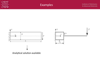
Figure 30: Cantilever beam subjects to an end shear force: discretisation of the solid
Figure 31: Cantilever beam subjects to an end shear force: von Mises stress di
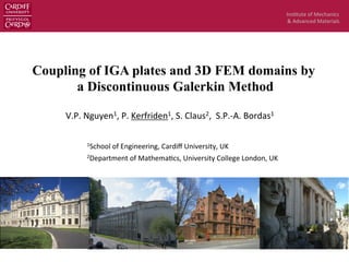
6.2.3. Non-conforming coupling of a square plate
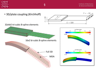
We consider a square plate of dimension L ⇥ L ⇥ t (t denotes the thickness) in which there
dimension Ls ⇥ Ls ⇥ t as shown in Fig. 32. In the computations, material properties are taken
the geometry data are L = 400, t = 20 and Ls = 100. The loading is a gravity force p = 10
is fully clamped. The stabilisation parameter was chosen empirically to be 1 ⇥ 106
. We us
NURBS plate elements for the plate and NURBS solid elements for the solid. In order to m
[Nguyen
et
al.
2013]
6.2.2. Cantilever plate: non-conforming coupling
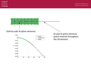
A mesh of 32 ⇥ 4 ⇥ 5/ 32 ⇥ 2 cubic elements is utilized for the mixed dimensional model, cf. F
the continuum part in the continuum-plate model is 175 mm. The contour plot of the von Mises s
where void plate elements were removed in the visualisation.
Figure 30: Cantilever beam subjects to an end shear force: discretisation of the solid an
Figure 31: Cantilever beam subjects to an end shear force: von Mises stress distrib
6.2.3. Non-conforming coupling of a square plate
We consider a square plate of dimension L ⇥ L ⇥ t (t denotes the thickness) in which there is a
CAD
model
Analysis
mesh
IGA
/
plate
Solid
FE
???

4. Ins$tute
of
Mechanics
&
Advanced
Materials
Figure 8. Stress contours in 3D–2D mixed-dimensional cantilever model loaded by a terminal
shear force Fz. (2D contours illustrated relate to top surface of model). Abaqus C3D20R brick
elements and S8R shell elements.
Figure 9. Transverse shear stresses 13 ( xz) obtained by method of Reference [5].
Copyright ? 2000 John Wiley & Sons, Ltd. Int. J. Numer. Meth. Engng 2000; 49:725–750
• Reference
coupling
§ displacement-­‐recovery,
Stress-­‐recovery
§ Equality
of
work
provides
coupling
on
dual
quan$ty
• Discrete
treatment
§ Mul$-­‐point
constraints
[Monaghan et al 1998,
McCune et al. 2000, Shim et al. 2002, Song et al. 2012]
§ Transi$on
elements
[Surana 1979, Cofer 1991,
Gmur et al, 1993, Dohrmann et al. 1999, Wagner et al. 2000,
Garusi et al. 2002, Chavan et al. 2004]
§ Mortar
methods
- Penalty
formula$ons
[Blanco et al. 2007]
- Lagrange
mul$plier-­‐based
mortar
[Rateau et al. 2003, Combescure et al. 2005]
- Hybrid
itera$ve
method
[Guguin et al. 2013]
Some
coupling
methods
in some situations.
3 Finite element formulation
Based on the above described kinematical assumptions the element is d
node in the transition cross–section is called ’reference node’. Furtherm
A2 and A3 define the orientation of the cross section. It is assumed th
couple (’coupling nodes’) lie in this plane. The vectors A2 and A3 are
section coordinates, see eq. (3). In the current configuration the base
the beam element together with the convective coordinates (0, ξ2, ξ3) a
define the coupling nodes.
The mechanical model of the cross section can be considered as a sum
allow only for axial deflections. The boundary conditions are clamped a
and jointed at the coupling node, see Fig. 3.
clamped bounded
rigid beam, axial free
hinged bounded
Transition elements
Fig. 3: Transition elements in a beam cross–section
The implementation of the constraint equation (7) in a transition elem
Penalty and the Augmented Lagrange Method. Furthermore a consi
derived for the element with respect to finite rotations. The transition is
Adapted
from
[Wagner
et
al.
2000]
lumique, qui occupent respectivement l’adh´erence des ouverts conn
commodit´e, nous d´esignons par !coq la surface moyenne du premier
sous-domaine correspondant de !0
. En outre, comme au §5.1.2.1, n
voisinage de la condition d’encastrement est repr´esent´e par le mod`ele
ωcoq
ω3d
sc
Fig. 5.8 – Mod´elisation Arlequin
Les relations de comportement sont celles des paragraphes 5.1.1.3 et 5.
champs de d´eplacement cin´ematiquement admissibles du mod`ele trid
par (5.17), tandis que celui du mod`ele coque est donn´e par l’expressio
W coq =
n
vcoq = v0
+ ⇠3(v1
⌧1 + v2
⌧2) ; v0
2 H1
(!0
coq), v1
, v2
2 H1
(!
106
[Rateau
et
al.
2003]
[McCune
et
al.
2000]

5. Ins$tute
of
Mechanics
&
Advanced
Materials
• Introduc$on
• Automa$c
coupling
§ Problem
statement
§ IGA
§ Discrete
coupling
strategy
• Numerical
examples
• Conclusion

6. Ins$tute
of
Mechanics
&
Advanced
Materials
§ Kinema$cs:
§ Equilibrium:
§ Cons$tu$ve
rela$on:
§ Primal
vibra$onal
formula$on:
Problem
statement:
uncoupled
solid
Figure 2: Coupling of a two dimensional solid and a beam.
as
(us
, us?
) :=
Z
⌦s
✏(u) : Cs
: ✏(us?
) d⌦ = ls
(us?
)
KA0
Z
⌦s
s
: ✏s
(us?
) d⌦ =
Z
⌦s
b · us?
d⌦ +
Z
t
¯t · us?
d
s
= Cs
: ✏s
in ⌦s
✏s
=
1
2
(rus
+ rT
us
)
us
= ¯u on s
u

7. Ins$tute
of
Mechanics
&
Advanced
Materials
§ Kinema$cs:
§ Equilibrium:
§ Cons$tu$ve
rela$on:
§ Primal
VF:
Problem
statement:
uncoupled
beam
Figure 2: Coupling of a two dimensional solid and a beam.
Z
⌦b
✓
N
M
◆
·
✓
v?
,¯x
w?
,¯x¯x
◆
dl =
Z
⌦b
0
@
¯p,¯x
¯p,¯y
¯m
1
A ·
0
@
v?
w?
w?
,¯x
1
A dl +
X
P 2Pntm
0
@
¯N
¯T
¯M
1
A
|P
·
0
@
v?
w?
w?
,¯x
1
A
|P
✓
N
M
◆
=
✓
ES 0
0 EI
◆ ✓
v,¯x
w,¯x¯x
◆
in ⌦b
v = ¯v on b
v
w = ¯w on b
w
w,¯x = ¯✓ on b
✓
ab
(⇥, ⇥b?
) :=
Z
⌦b
✓
v?
,¯x
w?
,¯x¯x
◆T ✓
ES 0
0 EI
◆
·
✓
v,¯x
w,¯x¯x
◆
dl = lb
(⇥b?
)
KA0

8. Ins$tute
of
Mechanics
&
Advanced
Materials
• Solid:
• EB-­‐Beam,
use
as
test
and
trial
in
2D
VF
Primal
coupling
(strong/weak)
as
(us
, us?
) = ls
(us?
) +
Z
?
us?
· ( s
(us
) · ns
) d
ab
(⇥b
, ⇥b?
) = lb
(⇥b?
) +
Z
?
ub
(⇥b?
) · ( b
(⇥b
) · nb
) d
ub
(⇥b
) =
✓
v w,¯x ¯y
w
◆
¯R

9. Ins$tute
of
Mechanics
&
Advanced
Materials
• Solid:
• EB-­‐Beam,
use
as
test
and
trial
in
2D
VF
• Primal
coupling
§ Kinema$cs:
- For
us:
§ V.
Work
equality
for
any
KA
field:
Primal
coupling
(strong/weak)
as
(us
, us?
) = ls
(us?
) +
Z
?
us?
· ( s
(us
) · ns
) d
ab
(⇥b
, ⇥b?
) = lb
(⇥b?
) +
Z
?
ub
(⇥b?
) · ( b
(⇥b
) · nb
) d
Choice
for
space?
For
us
Z
?
ub?
· ( s
(us
) · ns b
(⇥b
) · ns
) d = 0
ub
(⇥b
) =
✓
v w,¯x ¯y
w
◆
¯R
Figure 2: Coupling of a two dimensional solid and a beam.
Z
?
us
ub
(⇥) · ?
d
us
= ub
(⇥)

10. Ins$tute
of
Mechanics
&
Advanced
Materials
• Introduc$on
• Automa$c
coupling
§ Problem
statement
§ IGA
§ Discrete
coupling
strategy
• Numerical
examples
• Conclusion

11. Ins$tute
of
Mechanics
&
Advanced
Materials
B-­‐splines

12. Ins$tute
of
Mechanics
&
Advanced
Materials
Descrip$on
of
geometry
by
B-­‐splines
00.10.20.
0
0.1
0.2
0.3
0.4
0.5
0.6
0.7
0 0.1 0.2 0.3 0.4 0.5 0.6 0.7 0.8 0.9 1
0
0.1
0.2
0.3
0.4
0.5
0.6
0.7
0
0.1
0.2
0.3
0.4
0.5
0.6
0.7
0.8
0.9
0
0.1
0.2
0.3
0.4
0.5
0.6
0.7
0.8
0.9
1
0
0.05
N3,3(ξ)
M3,3(η)
Figure 4: A bivariate cubic B-spline basis function with knots vectors Ξ = H = {0, 0, 0, 0, 0.25, 0.5
ξ
η
x
y
z
(ξ, η)
0, 0, 0
0,0,0
1, 1, 1
1,1,1
0.5
0.5
Figure 5: A bi-quadratic B-spline surface (left) and the corresponding parameter space (right).
Ξ = H = {0, 0, 0, 0.5, 1, 1, 1}. The 4 × 4 control points are denoted by red filled circles.
12
⌅ = {⇠1, ⇠2, . . . , ⇠n+p+1}
x(⇠) =
nX
i
Ni,p(⇠) Bi
x(⇠, ⌘) =
nX
i
mX
j
Ni,p(⇠)Mj,p(⌘) Bij

13. Ins$tute
of
Mechanics
&
Advanced
Materials
IsoGeometric
Analysis
(IGA)
−0.5 0 0.5 1
−0.5
0
0.5
1
1.5
00.511.5
0 0.1 0.2 0.3 0.4 0.5 0.6 0.7 0.8 0.9 1
0
0.1
0.2
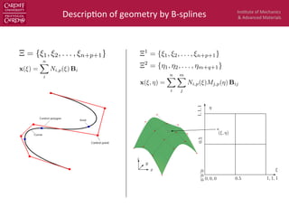
ariate cubic B-spline basis function with knots vectors Ξ = H = {0, 0, 0, 0, 0.25, 0.5, 0.75, 1, 1, 1, 1}.
ξ
η
x
y
z
(ξ, η)
0, 0, 0
0,0,0
1, 1, 1
1,1,1
0.5
0.5
uadratic B-spline surface (left) and the corresponding parameter space (right). Knot vectors are
0.5, 1, 1, 1}. The 4 × 4 control points are denoted by red filled circles.
12
⌅1
= {0, 0, 0, 0.5, 1, 1, 1}
⌅2
={0,0,0,0.5,1,1,1}
N2,3(⇠)
u(x(⇠, ⌘)) =
X
i
X
j
Ni,p(⇠)Mj,p(⌫)Uij
1
1
1
1 ¯⇠
ˆ⌦1 ˆ⌦2
ˆ⌦3 ˆ⌦4
¯⌘
⌘
⇠
0 0.5 1
1
0.5
Parametric
domain
Physical
domain
Parent
domain
(integra$on)
x(⇠, ⌘) =
nX
i
mX
j
Ni,p(⇠)Mj,p(⌘) Bij M2,2(⌘)
(⇠, ⌘)|ˆ⌦i = ˜((¯⇠, ¯⌘))
References:
[Kagan
et
al.
1998,
Cirak
et
al.
2000,
Hughes
et
al.
2005,
Cofrell
et
al.
2009]

14. Ins$tute
of
Mechanics
&
Advanced
Materials
• Introduc$on
• Automa$c
coupling
§ Problem
statement
and
reference
§ IGA
§ Discrete
coupling
strategy
• Numerical
examples
• Conclusion

15. Ins$tute
of
Mechanics
&
Advanced
Materials
• Penalty
formula$on
§
Mortaring
non-­‐conforming
discrete
spaces
JXK = Xs
Xb
us
= ub
(⇥)
In
discrete
space,
poten$ally
discon$nuous
a ⌘ as
+ ab
u ⌘ (us
, ⇥b
)ap
(uh
, u?
) =: a(uh
, u?
) + ↵
Z
?
Juh
K · Ju?
K d = l(u?
)

16. Ins$tute
of
Mechanics
&
Advanced
Materials
• Penalty
formula$on
§
§ Lack
of
consistency:
Mortaring
non-­‐conforming
discrete
spaces
JXK = Xs
Xb
hXi = Xs
+ (1 )Xb
us
= ub
(⇥)
In
discrete
space,
poten$ally
discon$nuous
J( · ns
) · u?
K = J · ns
K · hu?
i + Ju?
K h · ns
i
a ⌘ as
+ ab
u ⌘ (us
, ⇥b
)
=
1
2
ap
(uex
, u?
) l(u?
) =
Z
?
J (uex
) · ns
· u?
K 6= 0
ap
(uh
, u?
) =: a(uh
, u?
) + ↵
Z
?
Juh
K · Ju?
K d = l(u?
)

17. Ins$tute
of
Mechanics
&
Advanced
Materials
• Penalty
formula$on
§
§ Lack
of
consistency:
§ Nitsche
method:
add
to
penalty
formula$on
and
symmetrise
Mortaring
non-­‐conforming
discrete
spaces
JXK = Xs
Xb
hXi = Xs
+ (1 )Xb
us
= ub
(⇥)
In
discrete
space,
poten$ally
discon$nuous
an
(uh
, u?
) = a(uh
, u?
)
Z
?
Ju?
K
⌦
(uh
) · ns
↵
d
Z
?
Juh
K h (u?
) · ns
i d + ↵
Z
?
Juh
K · Ju?
K d = l(u?
)
J( · ns
) · u?
K = J · ns
K · hu?
i + Ju?
K h · ns
i```
a ⌘ as
+ ab
u ⌘ (us
, ⇥b
)
=
1
2
ap
(uex
, u?
) l(u?
) =
Z
?
J (uex
) · ns
· u?
K 6= 0
ap
(uh
, u?
) =: a(uh
, u?
) + ↵
Z
?
Juh
K · Ju?
K d = l(u?
)

18. Ins$tute
of
Mechanics
&
Advanced
Materials
• Penalty
formula$on
§
§ Lack
of
consistency:
§ Nitsche
method:
add
to
penalty
formula$on
and
symmetrise
Mortaring
non-­‐conforming
discrete
spaces
JXK = Xs
Xb
hXi = Xs
+ (1 )Xb
us
= ub
(⇥)
In
discrete
space,
poten$ally
discon$nuous
an
(uh
, u?
) = a(uh
, u?
)
Z
?
Ju?
K
⌦
(uh
) · ns
↵
d
Z
?
Juh
K h (u?
) · ns
i d + ↵
Z
?
Juh
K · Ju?
K d = l(u?
)
J( · ns
) · u?
K = J · ns
K · hu?
i + Ju?
K h · ns
i
J( · ns
) · u?
K = J · ns
K · (I ⇧b
) hu?
i + Ju?
K h · ns
i
```
a ⌘ as
+ ab
u ⌘ (us
, ⇥b
)
=
1
2
ap
(uex
, u?
) l(u?
) =
Z
?
J (uex
) · ns
· u?
K 6= 0
ap
(uh
, u?
) =: a(uh
, u?
) + ↵
Z
?
Juh
K · Ju?
K d = l(u?
)

19. Ins$tute
of
Mechanics
&
Advanced
Materials
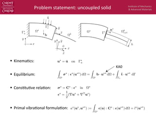
• Coercivity:
Stability
an
(uh
, u?
) = a(uh
, u?
)
Z
?
Ju?
K
⌦
(uh
) · ns
↵
d
Z
?
Juh
K h (u?
) · ns
i d + ↵
Z
?
Juh
K · Ju?
K d = l(u?
)
˜t(u) := (us
) + (ub
) · ns
in
discrete
space,
poten$ally
discon$nuous
Related work:
[Griebel et al. 2002,
Dolbow et al. 2009]
an
(u, u) = a(u, u) + ↵
Z
?
JuK · JuK d
Z
?
JuK · ˜t(u) d
an
(u, u) Cc
kuk2
X

20. Ins$tute
of
Mechanics
&
Advanced
Materials
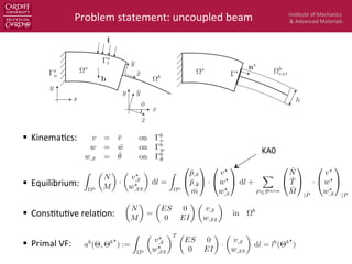
• Coercivity:
§ Parallelogram
ineq.
:
§ ``Trace
inequality”
(assump$on)
→
Stability
an
(uh
, u?
) = a(uh
, u?
)
Z
?
Ju?
K
⌦
(uh
) · ns
↵
d
Z
?
Juh
K h (u?
) · ns
i d + ↵
Z
?
Juh
K · Ju?
K d = l(u?
)
˜t(u) := (us
) + (ub
) · ns
k˜t(u)k2
?  C2
a(u, u)
an
(u, u)
✓
1
C2
✏
2
◆
a(u, u) +
✓
↵
1
2✏
◆
kJuKk2
?
in
discrete
space,
poten$ally
discon$nuous
✏ =
1
C2
) ↵ >
C2
2
Related work:
[Griebel et al. 2002,
Dolbow et al. 2009]
an
(u, u) a(u, u) + ↵kJuKk2
?
✓
1
2✏
kJuKk2
? +
✏
2
k˜t(u)k2
?
◆
an
(u, u) = a(u, u) + ↵
Z
?
JuK · JuK d
Z
?
JuK · ˜t(u) d
an
(u, u) Cc
kuk2
X

21. Ins$tute
of
Mechanics
&
Advanced
Materials
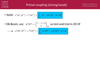
• Solve
numerically
for
regularisa$on
parameter
s.
t.
→
→
Eigenvalue
problem
for
regularisa$on
parameter
↵ >
1
2
Kuncoupled 1
H
a(u, u) = [u]T
Kuncoupled
[u]
k˜t(u)k2
? =
Z
?
( (us
) + (ub
)) · ns
· ( (us
) + (ub
)) · ns
d = [u]T
H [u]
1
largest
eigenvalue
of
Related work:
[Griebel et al. 2002,
Dolbow et al. 2009]
k˜t(u)k2
? < 2↵ a(u, u)
References on embedded interfaces and implicit boundaries using Nitsche [Hansbo et al. 2002,
Dolbow et al. 2009, Sanders et al. 2011, Burman et al. 2012, Chouly et al. 2013]
1
2
[u]T
H [u]
[u]T Kuncoupled [u]
< ↵

22. Ins$tute
of
Mechanics
&
Advanced
Materials
• Introduc$on
• Automa$c
coupling
§ Problem
statement
and
reference
§ IGA
§ Discrete
coupling
strategy
• Numerical
examples
• Conclusion

23. Ins$tute
of
Mechanics
&
Advanced
Materials
Examples
ux(x, y) =
Py
6EI

(6L 3x)x + (2 + ⌫)
✓
y2 D2
4
◆
uy(x, y) =
P
6EI

3⌫y2
(L x) + (4 + 5⌫)
D2
x
4
+ (3L x)x2
(88)
tresses are
xx(x, y) =
P(L x)y
I
; yy(x, y) = 0, xy(x, y) =
P
2I
✓
D2
4
y2
◆
(89)
tions, material properties are taken as E = 3.0 ⇥ 107
, ⌫ = 0.3 and the beam dimensions are D = 6 and
hear force is P = 1000. Units are deliberately left out here, given that they can be consistently chosen
In order to model the clamping condition, the displacement defined by Equation (88) is prescribed as
ary conditions at x = 0, D/2  y  D/2. This problem is solved with bilinear Lagrange elements (Q4
high order B-splines elements. The former helps to verify the implementation in addition to the ease of
Dirichlet boundary conditions (BCs). For the latter, care must be taken in enforcing the Dirichlet BCs
on (88) since the B-spline basis functions are not interpolatory.
Figure 13: Timoshenko beam: problem description.
continuum-beam model is given in Fig. 14. The end shear force applied to the right end point is F = P.
Figure 14: Timoshenko beam: mixed continuum-beam model.
ments In the first calculation we take lc = L/2 and a mesh of 40 ⇥ 10 Q4 elements (40 elements in the
n) was used for the continuum part and 29 two-noded elements for the beam part. The stabilisation
enforcement of Dirichlet boundary conditions (BCs). For the latter, care must be taken in enforcing the Dirich
given in Equation (88) since the B-spline basis functions are not interpolatory.
Figure 13: Timoshenko beam: problem description.
The mixed continuum-beam model is given in Fig. 14. The end shear force applied to the right end point is
Figure 14: Timoshenko beam: mixed continuum-beam model.
Lagrange elements In the first calculation we take lc = L/2 and a mesh of 40 ⇥ 10 Q4 elements (40 element
length direction) was used for the continuum part and 29 two-noded elements for the beam part. The stab
26
Analy$cal
solu$on
available
?

24. Ins$tute
of
Mechanics
&
Advanced
Materials
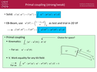
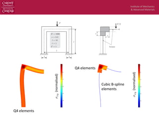
parameter ↵ according to Equation (55) was 4.7128 ⇥ 107
. Fig. 15a plots the transverse displacement (taken as nodal
values) along the beam length at y = 0 together with the exact solution given in Equation (88). An excellent agreement
with the exact solution can be observed and this verified the implementation. The comparison of the numerical stress
field and the exact stress field is given in Fig. 15b with less satisfaction. While the bending stress xx is well estimated,
the shear stress xy is not well predicted in proximity to the coupling interface. This phenomenon was also observed
in the framework of Arlequin method [64] and in the context of MPC method [38]. Explanation of this phenomenon
will be given subsequently.
0 10 20 30 40 50
−0.07
−0.06
−0.05
−0.04
−0.03
−0.02
−0.01
0
x
w
exact
coupling
(a) transverse displacement
0 5 10 15 20 25
−400
−200
0
200
400
600
800
x
stressesalongy=0.3
sigmaxx−exact
sigmaxx−coupling
sigmaxy−exact
sigmaxy−coupling
(b) stresses
Figure 15: Mixed dimensional analysis of the Timoshenko beam: comparison of numerical solution and exact solution.
Q4
elements
2-­‐noded
cubic
elements
Deflec$on
of
neutral
axis
Stress
profile

25. Ins$tute
of
Mechanics
&
Advanced
Materials
32x4
bi-­‐cubic
B-­‐spline
elements
8
cubic
B-­‐spline
elements
(patch
extends
throughout
the
2D
domain)
shenko beam: non-conforming coupling
ction, a non-conforming coupling is considered. The B-spline mesh is given in Fig. 21. Refined meshes are
m this one via the knot span subdivision technique. We use the mesh consisting of 32 ⇥ 4 cubic continuum
d 8 cubic beam elements. Fig. 22 gives the mesh and the displacement field in which lc = 29.97 so that
interface is very close to the beam element boundary. A good solution was obtained using the simple
scribed in Section 5.
Mixed dimensional analysis of the Timoshenko beam with non-conforming coupling. The continuum part
y 8 ⇥ 2 bi-cubic B-splines and the beam part is with 8 cubic elements.
−0.06
−0.05
−0.04
−0.03
−0.02
−0.01
0
0.01
w
exact
continuum
beam
orming coupling
g coupling is considered. The B-spline mesh is given in Fig. 21. Refined meshes are
span subdivision technique. We use the mesh consisting of 32 ⇥ 4 cubic continuum
ts. Fig. 22 gives the mesh and the displacement field in which lc = 29.97 so that
to the beam element boundary. A good solution was obtained using the simple
ysis of the Timoshenko beam with non-conforming coupling. The continuum part
es and the beam part is with 8 cubic elements.
0 10 20 30 40 50
−0.07
−0.06
−0.05
−0.04
−0.03
−0.02
−0.01
0
0.01
x
w
exact
continuum
beam
(b) displacement field
ysis of the Timoshenko beam with non-conforming coupling: (a) 32 ⇥ 4 Q4 elements
ts and (b) displacement field.

26. Ins$tute
of
Mechanics
&
Advanced
Materials
dofs. The total number of dofs of the continuum-beam model is only 5400. The stabilisation parameter is taken to be
↵ = 107
and used for both coupling interfaces. A comparison of xy contour plot obtained with (1) and (2) is given in
Fig. 25. A good agreement was obtained.
Figure 23: A plane frame analysis: problem description.
Remark 6.1. Although the processing time of the solid-beam model is much less than the one of the solid model, one
cannot simply conclude that the solid-beam model is more e cient. The pre-processing of the solid-beam model, if not
automatic, can be time consuming such that the gain in the processing step is lost. For non-linear analyses, where the
processing time is dominant, we believe that mixed dimensional analysis is very economics.
6.2. Continuum-plate coupling
6.2.1. Cantilever plate: conforming coupling
For verification of the continuum-plate coupling, we consider the 3D cantilever beam given in Fig. 26. The material
properties are E = 1000 N/mm2
, ⌫ = 0.3. The end shear traction is ¯t = 10 N/mm in case of continuum-plate model
and is ¯t = 10/20 N/mm2
in case of continuum model which is referred to as the reference model. We use B-splines
elements to solve both the MDA and the reference model. The length of the continuum part in the continuum-plate
model is L/2 = 160 mm. A mesh of 64 ⇥ 4 ⇥ 5 tri-cubic elements is utilized for the reference model and a mesh of
32 ⇥ 4 ⇥ 5/ 16 ⇥ 2 cubic elements is utilized for the mixed dimensional model, cf. Fig. 27. The plate part of the
mixed dimensional model is discretised using the Reissner-Mindlin plate theory with three unknowns per node and the
Kirchho↵ plate theory with only one unknown per node. The stabilisation parameter was chosen empirically to be
5⇥103
. Note that the eigenvalue method described in Section 4.3 can be used to rigorously determine ↵. However since
it would be expensive for large problems, we are in favor of simpler but less rigorous rules to compute this parameter.
Fig. 28 shows a comparison of deformed shapes of the continuum model and the continuum-plate model and in Fig. 29,
the contour plot of the von Mises stress corresponding to various models is given.
31
Figure 24: A plane frame analysis: solid-beam model.
Figure 25: A plane frame analysis: comparison of xy contour plot obtained with solid model (left) a
model (right).
Figure 24: A plane frame analysis: solid-beam model.
xy(normalised)
xy(normalised)
Q4
elements
Q4
elements
Cubic
B-­‐spline
elements

27. Ins$tute
of
Mechanics
&
Advanced
Materials
27: Cantilever beam subjects to an end shear force: typical B-spline discretisation.
r beam subjects to an end shear force: comparison of deformed shapes of the continuum model
• 3D/plate
coupling
(Kirchhoff)
§
Figure 25: A plane frame analysis: comparison of xy contour plot obtained with solid mode
model (right).
Figure 26: Cantilever beam subjects to an end shear force: problem setup
32
27: Cantilever beam subjects to an end shear force: typical B-spline discretisation.
10.0 20.0 30.0 40.0 50.0
von Mises stress
0.429 51
(a) reference model
10.0 20.0 30.0 40.0
von Mises stress
5.17 48.6
(b) mixed dimensional model, Mindlin plate
10.0 20.0
von Mis
5.12
(c) mixed dimensional
10.0 20.0 30.0 40.0 50.0
von Mises stress
0.429 51
(a) reference model
10.0 20.0 30.0 40.0
von Mises stress
5.17 48.6
(b) mixed dimensional model, Mindlin plate
10.0 20.0 30.0 40.0
von Mises stress
5.12 48.6
(c) mixed dimensional model, Kirchho↵ plate
32x4x5
tri-­‐cubic
B-­‐spline
elements
16x2
bi-­‐cubic
B-­‐spline
elements
Full
3D
MDA

28. Ins$tute
of
Mechanics
&
Advanced
Materials
ure 32: Square plate enriched by a solid. The highlighted elements are those plate elem
undaries. The plate is fully clamped ans subjected to a gravity force.
ments with some geometry entities is popular in XFEM, see e.g., [58]. Fig. 33 plots the de
the solid-plate model and the one obtained with a plate model. A good agreement can be o
w the flexibility of the non-conforming coupling, the solid part was moved slightly to the rig
figuration is given in Fig. 34. The same discretisation for the plate is used. This should ser
del adaptivity analyses to be presented in a forthcoming contribution.
ure 33: Square plate enriched by a solid: transverse displacement plot on deformed configur
ate enriched by a solid. The highlighted elements are those plate elements cut by the s
is fully clamped ans subjected to a gravity force.
eometry entities is popular in XFEM, see e.g., [58]. Fig. 33 plots the deformed configura
el and the one obtained with a plate model. A good agreement can be observed. In orde
the non-conforming coupling, the solid part was moved slightly to the right and the defor
in Fig. 34. The same discretisation for the plate is used. This should serve as a prototype
yses to be presented in a forthcoming contribution.
te enriched by a solid: transverse displacement plot on deformed configurations of plate m
Figure 32: Square plate enriched by a solid. The highlighted elements are those plate elements cut by the solid
boundaries. The plate is fully clamped ans subjected to a gravity force.
elements with some geometry entities is popular in XFEM, see e.g., [58]. Fig. 33 plots the deformed configuration
of the solid-plate model and the one obtained with a plate model. A good agreement can be observed. In order to
show the flexibility of the non-conforming coupling, the solid part was moved slightly to the right and the deformed
configuration is given in Fig. 34. The same discretisation for the plate is used. This should serve as a prototype for
model adaptivity analyses to be presented in a forthcoming contribution.
Load:
weight
Fully
clamped

29. Ins$tute
of
Mechanics
&
Advanced
Materials
• Versa$le
coupling
for
mixed-­‐dimensional
analysis
with
non-­‐conforming
discre$sa$ons
(IGA/FEM)
• Future
work
§ Weighted
averages
in
the
Nitsche
Plate/3D
coupling
§ Cheap
way
to
evaluate
the
lower
bound
on
the
regularisa$on
parameter
§ Efficient
and
weakly
intrusive
local/global
solver
§ Damage
in
solid
region
Conclusion