J012546068

IOSR Journal of Mechanical and Civil Engineering (IOSR-JMCE)
e-ISSN: 2278-1684,p-ISSN: 2320-334X, Volume 12, Issue 5 Ver. IV (Sep. - Oct. 2015), PP 60-68
www.iosrjournals.org
DOI: 10.9790/1684-12546068 www.iosrjournals.org 60 | Page
Soil Structure Interaction Calculus, For Rigid Hydraulic
Structures, Using FEM
Costel Boariu
Department of Hydraulic Structures Engineering, Faculty Hydrotechnical Engineering, Geodesy and
Environmental Engineering, Gheorghe Asachi Technical University of Iași, Romania
Abstract: The interaction between the foundation and the deformable soil calculated by finite element method
is based on various models representing terrain behavior. Of these models, most commercial calculation
programs implemented in their content models Winkler and Pasternak. Article shows the influence of these
computing models on conventional rigid hydraulic construction. It was calculated the stiffness matrix structure
and deformations developed, by considering these two models.
Keywords: FEM, Pasternak model, rigid structure, stiffness matrix
I. Introduction
The traditional method for simulation the mathematical load-deformation response of a beam in
uniaxial bending is a differential equation (Horvath 2002) [1]. The basic form of the matrix formulation for
beam flexure is
    S d q (1)
where:
[S] = stiffness matrix; {d} = displacement vector; {q} = load (force) vector.
The relevance of equation (1) is that all of the variations in beam behavior can be explained as variations solely
in the formulation of the stiffness matrix, [S].
In Winkler model (Fig.1) the flexural behavior of this beam is given by equation (2)
V e rtic a l s o il s p rin g (p = k w )
B e a m (E , I)
lo a d q
l
w
x
Fig. 1 The Winkler model
4
4
( )
( ) ( )
d w x
E I p x q x
dx
  (2)
where subgrade reaction in one (x-axis) direction only is
( ) ( )w
p x k w x
kw = Winkler coefficient of subgrade reaction
E = elasticity modulus of beam
I = beam moment of inertia
Solving ecuation (2) by FEM is expressed by relation (3)
       e w
S S d q  (3)
wherein elastic stiffness matrix expression [Se] and subgrade reaction matrix [Sw] are determined with
the following shape function(4) according to Cook [2] Chang [3] Teodoru [4]
   
   
2 3 2 3
1 22 3 2
2 3 2 3
3 42 3 2
3 2 2
1 ; ;
3 2
; .
x x x x
N x N x x
ll l l
x x x x
N x N x
ll l l
     
    
(4)
Stiffness matrix are:

Soil Structure Interaction Calculus, For Rigid Hydraulic Structures, Using FEM
2 2
3
2 2
1 2 6 1 2 6
6 4 6 2 l
1 2 6 1 2 6
6 2 6 4
e
l l
l l lE I
S
l ll
l l l l
 
 
 
      
 
  
(5)
2 2
2 2
1 5 6 2 2 5 4 1 3
2 2 4 1 3 3
5 4 1 3 1 5 6 2 24 2 0
13 3 2 2 4
w
w
l l
l l l lk l
S
l l
l l l l
 
 
 
    
 
    
(6)
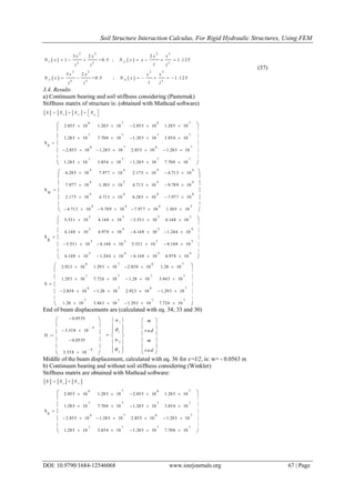
In Pasternak model (fig.2) The flexural behavior of this beam is given by equation (7)
4 2
4 2
( ) ( )
( ) ( )
d w x d w x
E I p x g q x
dx x
   (7)
where g = the shear stiffness of the shear layer. Solving ecuation (7) by FEM is expressed by relation (8)
       e w g
S S S d q   
 
(8)
wherein elastic stiffness matrix expression [Se] is subgrade reaction matrix [Sw] are the same like those
from relations (5) and (6) and matrix [Sg] is given by equation (9)
2 2
2 2
3 6 3 3 6 3
3 4 3
3 6 3 3 6 33 0
3 3 4
g
l l
l l l lg
S
l ll
l l l l
 
 
 
   
     
 
  
(9)
The introduction of second parameter for soil (shear stiffness) have the same effect like siffness grovth
of the beam (the terms of stiffness matrix is increase)
B e a m ( E , I)
lo a d q
l
w
x
S h e a r la y e r (g )
Fig. 2 The Pasternak model
Stiffness matrix is obtained considering continuum bearing on soil like in fig. 3
y
1 .0 x
E I
S 2 3
S 1 3
S 4 3
S 3 3
y
x
E IS 2 1
S 1 1
S 4 1
S 3 1
1 .0
y
x
E I
S 2 4
S 1 4
S 4 4
S 3 4
1 .0
k w
k wk w
y
x
E I S 4 2
S 3 2
S 2 2
S 1 2
1 .0
k w
l l
ll
Fig. 3 Stiffness matrix calculation by continuum bearing

II. Stiffness Matrix Calculation By Punctual Bearing Of The Beam
In beam on elastic foundation calculus by FEM, subgrade reaction matrix of Winkler spring was given
by Bowles [5] in configuration (10)
1 0 0 0
0 0 0 0
0 0 1 02
0 0 0 0
w
w
k l
S
 
 
   
 
 
 
(10)
This expression is direct suggestion by calculus scheme from fig. 4, where can be see that only
elements S11 and S33 of stiffness matrix have values different of zero values. (There's an element stiffness matrix
Sij is generalized force that develops on i direction when in the direction of j is imposed on movement or
rotation unit)
y
1 .0 x
E I
S 2 3
S 1 3
S 4 3
S 3 3
y
x
E IS 2 1
S 1 1
S 4 1
S 3 1
1 .0
y
x
E I
S 2 4
S 1 4
S 4 4
S 3 4
1 .0
k w
k w ·l/2
y
x
E I S 4 2
S 3 2
S 2 2
S 1 2
1 .0
l l
l l
k w ·l/2
k w ·l/2 k w ·l/2
Fig. 4 Stiffness matrix calculation by nodal bearing
In ecuation (7) apart from term which include Winkler springs and for which stiffness matrix member
S11 and S33 are easy to find (intuit) , apear and terms which include shearing efect for which stiffness matrix
intuition is not simple. The term of the equation that considers the earth shear, contain second derivative of
beam deformation(d2
w/dx2
). To calculate the stiffness matrix expressing shear earth [Sg] in case of nodal
bearing, on use similar functions to those for calculating matrix form [Sw]
Relation (10) for [Sw] rezult by solving with Galerkin method of differential ecuation (7)
Seeing that expression we(x) = N1(x)w1+N2(x)θ1+N3(x)w2+N4(x)θ2 (11)
is an approximal solution of differential ecuation (7) it rezult an residuum
4 2
4 2
( ) ( )
( ) ( ) ( ) 0
e e
e
d w x d w x
x E I g kw x q x
dx x
      (12)
in which k=kw·1 considering an unitar width beam or k=kw·B for a beam of B width; after Chung [6]
With this reziduum on form balanced reziduum functionals with shape functions
     
 
4 2
4 2
0 0 0
0 0
( ) ( )
, ( )
( ) ( ) ( ) 0
l l l
e e
i i i i
l l
i e i
d w x d w x
N x x t d x E I N x d x g N x d x
d x d x
k N x w x d x N x q x d x
      
  
  
 
(13)
From first integral of expresion (13) on obtain nodal force vector and elastic stiffness matrix of the
beam(5). From the third integral obtain subgrade reaction matrix of Winkler spring, considring relation (11)
write in form: w(x)=[N(x)]{de}, cu {de}={w1 θ1 w2 θ2}
     
1
2
1 2 3 4
30 0 0
4
( )
( )
( ) ( ) ( ) ( ) ( ) ( )
( )
( )
l l l
w i e i j
N x
N x
S k N x w x d x k N x N d x k N x N x N x N x d x
N x
N x
 
 
   
 
 
 
   (14)
Following stiffness matrix became

 
 
 
 
2
1 1 2 1 3 1 4
2
2 1 2 2 3 2 4
2
0 3 1 3 2 3 3 4
2
4 1 4 2 4 3 4
l
w
N N N N N N N
N N N N N N N
S k d x
N N N N N N N
N N N N N N N
 
 
 
 
   
 
 
 
 
 
 (15)
In relation (15) if accepted for shape function the relations(16)
1 ( )N x 
1,
2
0,
2
l
x
l
x l

 
;  2 ( ) 0, 0,N x x l  (16)
3 ( )N x 
0,
2
1,
2
l
x
l
x l

 
;  4 ( ) 0, 0,N x x l 
subgrade reaction matrix of Winkler spring become
0 0 0
2
0 0 0 0
0 0 0
2
0 0 0 0
w
l
S k
l
 
 
 
 
    
 
 
 
 
(17)
In this way was find the same subgrade reaction matrix of Winkler spring, like that given by
Bowles(1996)
Folowing on use shape function for matrix [Sg] calculation
If from ecuation (13) using the first two integral and consider shear stress attached to g parameter ,
after Zhaohua apud Teodoru [4]
3
3
e e
d w d w
E I Q g
d xd x
 
obtain integration by parts
   
   
3 2 2
'
3 2 2
00 0 0 0
2
'' '
200
0 00 0
'( ) ''( ) ( )
( ) ( ) ( ) ( ) ( ) ( )
l l l ll
e e e e
i i i i i
l ll l
l le e e e
i i i i i i
d w d w d w d wd w
N x E I N x E I E I N x d x g N x g N x d x
d x d xd x d x d x
d w d w d w d w
N x Q x g N x N x M x E I N x d x g N x g N x d x
d x d x d xd x
    
     
 
 
(18)
From ecuation (18) the last member give stiffness matrix wich simulate shear stres in soil
 
'
1
'
' ' ' ' ' ' '2
1 2 3 4'
30 0 0
'
4
( )
( )( )
( ) ( ) ( ) ( ) ( )
( )
( )
l l l
e
g i i j
N x
N xd w x
S g N x d x g N x N d x g N x N x N x N x d x
d x N x
N x
 
 
       
    
 
  
   (19)
Forward stiffness matrix become
 
 
 
 
2
' ' ' ' ' ' '
1 1 2 1 3 1 4
2
' ' ' ' ' ' '
2 1 2 2 3 2 4
2
' ' ' ' ' ' '
0 3 1 3 2 3 3 4
2
' ' ' ' ' ' '
4 1 4 2 4 3 4
l
g
N N N N N N N
N N N N N N N
S g d x
N N N N N N N
N N N N N N N
 
 
 
 
   
   
 
 
 
 
 (20)
where („) denotes differentiation with respect to x

If using shape functions (16) like those used for subgrade reaction matrix of Winkler spring
calculation, [Sw] (17) , shear matrix is [Sg] = 0
If using for matrix [Sw] calculation linear shape function (21)
1 2 3 4( , ) 1 , ( ) 0, ( ) , N ( ) 0
x x
N x t N x N x x
l l
     (21)
it obtain the folowing stiffness matrix
2 0 1 0
0 0 0 0
1 0 2 06
0 0 0 0
w
kl
S
 
 
   
 
 
 
(22)
1 0 1 0
0 0 0 0
1 0 1 0
0 0 0 0
g
g
S
l
 
 
   
   
 
 
(23)
Stiffness matrix obtained with relation (22) and (23) as well those given by (17) and Sg=0 are very
approximal because of rough shape function expresion used (16) and (21).
In folowing example on use the interaction model with continuum bearing. The goal of calculus example is to
find stiffness matrix and displacements for a special structure with large rigidity
III. Calculus Example
3.1. Design structure and calculus schedule
The structure is bottom discharge at an earth dam(Ibaneasa dam from Botosani county – Romania).
The conduit is made by steel concrete with polygonal cross section (fig. 5) - internal quadratic and external
trapezoid.
3 .2 0
2 .6 0
1 .7 0
2 .3 0
4 5
4 5
3 .2 0
9 .0 0
S id e s e e p a g e s to p
Fig. 5 Cross and longitudinal section by bottom discharge (concrete steel)
The conduit is separated in 9m length transom. It shall be calculate a central transom of bottom
discharge.
The load and bearing schedule is in fig. 6. It shall be consider a sigle beam finit element between two
joints with length l
3.2. Earth (soil) and beam (conduit) parameters
The conduit parameters are:
A=5.36 m2
; Ib=6.67 m4
; Eb=26 GPa (for C12/15 concrete)
The ground under conduit
Each node will be thought of as a spring with its elasticity determined according to Chung [ ] by :
ks = B· k in which
B = 3.2 m is the width of the conduit

B e a m (E , I)
lo a d q
l
w
x
V e rtic a l s o il s p rin g (p = k ·l/2 ·w )
B e a m (E , I)
lo a d q
l
w
x
a ) c o n tin u u m b e a rin g
b ) te rm in a l p o in ts b e a rin g
Fig. 6 Beam loading schedule
The marginal nodes will have the same coefficient of subgrade reaction as the other ones according to
Bowles
Coefficient of subgrade reaction according to Vesić apud Bowles [5]
4
1 2
2
0 .6 5
(1 )
p p
b b p
E B E
k
E I B 


(24)
Ground parameters are (silty clay):
Ep=35 MPa; μp=0,35; γp=19 kN/m3
4
1 2
2
3 5 3 .2 3 5
0 .6 5 5 8 7 5
2 6 0 0 0 6 .6 7 3 .2 (1 0 .3 5 )
k

 
 
kN/m3
ks = 3.2 · 5875 = 28 200 kN/m;
Shear modulus for shear layer in foundation is
2 (1 )
p
p
E
g



= 13 Mpa (25)
gs= B· g
Foundation parameters k and g may be calculated according Horvath [7] with following relations
p
E
k
H
 (26)
2 (1 ) 2
p
p
E H
g



(27)
where H is depth to effective rigid base
The effective rigid base is defined as the depth at which settlements caused by the structure can be
taken to be zero. For decades it has been assumed that the “depth of influence” for settlement equivalent
conceptually to the effective depth to rigid base is twice the width of a square loaded area and four times the
width of an infinite strip-Colasanti and Horvath [8]
With this assumptions H=6,4 m ; k=5468 kN/m2
; g=41,5 MPa
Earth load on conduit may be consider uniform distributed (crown width is 6 m and conduit beam
length is 9 m).
Earth load together with self weight of conduit is q=826 kN/m
With this parameter it shall be calculate structure wich schedule is presented in fig 6
3.3. Solving equilibrium equation sistem
Matrix equation is (8)        e w g
S S S d q   
 
, whitch write like (1) is
    S D Q
in which members are:
     e w g
S S S S   
  = stiffness matrix
{D}={d} = displacement vector
{Q}={q} = load (force) vector.
Solving ecuation (1) is by partitioning matrix S; D and Q whereby it separate out free displacement for degree
of freedom (2 and 4) by degree of freedom with elastic bearings (1 and 3)- Jerca [9], see Fig 7

n n n r n n n
rn rr r r r
S S D Q R
S S D Q R
       
       
      
(28)
n n n n r r n n
rn n rr r r r
S D S D Q R
S D S D Q R
  
  
(29)
Fig. 7 Beam displacements (degrees of freedom)
1 1
2 2
;n r
w
D D
w


   
    
   
are displacement vectors
2
2
1 2 2
21 2
n r
l l
Q q Q q
ll
   
       
    
   
     
are load vectors
1 12
3 34
0
;
0
n r s s r
R dR
R R k k D
R dR
      
           
      
(30)
are reaction in degree of freedom directions
or (with the same result)  
1 1
3 3
0
0
s
r s r
s
R k d
R k D
R k d
     
      
     
(31)
Replacing eq (30) writen like
1
r r
s
D R
k
 , in eq (29) obtain
1
1
( )
nn n nr r n
s
rn n rr r r
s
S D S R Q
k
S D S I R Q
k
 
  
(32)
From last ecuation result
11
( ) ( )r rr r rn n
s
R S I Q S D
k

   (33)
wich indroducing in first one, guide to displacement calculation
11 1
( ) ( )nn n nr rr r rn n n
s s
S D S S I Q S D Q
k k

    ; 1 11 1 1 1
( ) ( )nn n nr rr r nr rr rn n n
s s s s
S D S S I Q S S I S D Q
k k k k
 
    
1 11 1 1 1
[ ( ) ] ( )nn nr rr rn n n nr rr r
s s s s
S S S I S D Q S S I Q
k k k k
 
    
Displacement in free(no bearing) degree of freedom directions(2 and 4, Fig. 6) are
 
1
* *
n nn n
D S Q

 in wich (34)
* 1 * 11 1 1 1
( ) ; ( )nn nn nr rr rn n n nr rr r
s s s s
S S S S I S Q Q S S I Q
k k k k
 
     
After ends of beam displacement calculation it shall be calculated middle of the beam displacement
with next relation:
we(x=l/2) = N1(x)w1+N2(x)θ1+N3(x)w2+N4(x)θ2 (35)
which in matrix shape is:
  w N d (36)
in which shape function for x=l/2 are (4 equations)

1
1
2
2
w
w


 
 
 
  
 
 
 
m
ra d
m
ra d
 
 
 
 
 
 
   
   
2 3 2 3
1 22 3 2
2 3 2 3
3 42 3 2
3 2 2
1 = 0 .5 ; 1 .1 2 5
3 2
= 0 .5 ; 1 .1 2 5
x x x x
N x N x x
ll l l
x x x x
N x N x
ll l l
      
      
(37)
3.4. Results
a) Continuum bearing and soil stiffness considering (Pasternak)
Stiffness matrix of structure is: (obtained with Mathcad software)
     e w g
S S S S   
 
S
e
2.855 10
6

1.285 10
7

2.855 10
6

1.285 10
7

1.285 10
7

7.708 10
7

1.285 10
7

3.854 10
7

2.855 10
6

1.285 10
7

2.855 10
6

1.285 10
7

1.285 10
7

3.854 10
7

1.285 10
7

7.708 10
7
















S
w
6.285 10
4

7.977 10
4

2.175 10
4

4.713 10
4

7.977 10
4

1.305 10
5

4.713 10
4

9.789 10
4

2.175 10
4

4.713 10
4

6.285 10
4

7.977 10
4

4.713 10
4

9.789 10
4

7.977 10
4

1.305 10
5
















S
g
5.531 10
3

4.148 10
3

5.531 10
3

4.148 10
3

4.148 10
3

4.978 10
4

4.148 10
3

1.244 10
4

5.531 10
3

4.148 10
3

5.531 10
3

4.148 10
3

4.148 10
3

1.244 10
4

4.148 10
3

4.978 10
4
















S
2.923 10
6

1.293 10
7

2.838 10
6

1.28 10
7

1.293 10
7

7.726 10
7

1.28 10
7

3.843 10
7

2.838 10
6

1.28 10
7

2.923 10
6

1.293 10
7

1.28 10
7

3.843 10
7

1.293 10
7

7.726 10
7
















End of beam displacements are (calculated with eq. 34; 33 and 30)
D
0.0555
3.338 10
4

0.0555
3.338 10
4














Middle of the beam displacement, calculated with eq. 36 for x=l/2, is: w= - 0.0563 m
b) Continuum bearing and without soil stiffness considering (Winkler)
Stiffness matrix are obtained with Mathcad software:
     e w
S S S 
S
e
2.855 10
6

1.285 10
7

2.855 10
6

1.285 10
7

1.285 10
7

7.708 10
7

1.285 10
7

3.854 10
7

2.855 10
6

1.285 10
7

2.855 10
6

1.285 10
7

1.285 10
7

3.854 10
7

1.285 10
7

7.708 10
7

















1
1
2
2
w
w


 
 
 
  
 
 
 
m
ra d
m
ra d
 
 
 
 
 
 
S
w
6.285 10
4

7.977 10
4

2.175 10
4

4.713 10
4

7.977 10
4

1.305 10
5

4.713 10
4

9.789 10
4

2.175 10
4

4.713 10
4

6.285 10
4

7.977 10
4

4.713 10
4

9.789 10
4

7.977 10
4

1.305 10
5
















S
2.917 10
6

1.293 10
7

2.833 10
6

1.28 10
7

1.293 10
7

7.721 10
7

1.28 10
7

3.844 10
7

2.833 10
6

1.28 10
7

2.917 10
6

1.293 10
7

1.28 10
7

3.844 10
7

1.293 10
7

7.721 10
7
















End of beam displacements are
D
0.0563
3.372 10
4

0.0563
3.372 10
4














Middle of the beam displacement is: w = -0.0571 m
IV. Conclusions
Displacements in those two calculus hypothesis are very close (2% difference )
Shear stiffness of the soil considering in Pasternak hypothesis is inconsequent because of structure particulars.
This is possible due to the overall rigidity of the structure. The rigidity of one section is according to Gorbunov
Posadov [10] Paulos [11]
2 3 3
2 3
1 ( / 2 ) ( / 2 )
1 0
41
p pb
b bp
E EB B
t
E I E h
 


 

Given this data, we have t=0,0007<<1 so the conduit is (very)rigid.
The explanation lies in the rigidity of the bottom-discharge conduit structure. Thus the elastic stiffness
matrix of the structure is a little modified of rigidity matrix resulted by taking into consideration the specific
earth stiffness of the Pasternak model.
So for rigid structures, earth stiffness change (increase) settled by Pasternak hypotthesis and many
other researchers (Thangaraj [12], Tiwari [13]) is not suitable.
References
[1] Horvath John S., Soil-Structure Interaction Research Project (2002) www.engineering.manhattan.edu/civil/CGT.html.
[2] Cook R.,D., Finite Element Modeling for Stress Analysis, John Wiley & Sons, Inc. 1995
[3] Chang-Yu Ou, Deep Excavation. Theory and practice. Taylor & Francis/Balkena Leiden 2006
[4] Teodoru I.,B., Musat V., Soil structure interaction numerical modelling. Foundation beams Editura Politehnium Iasi 2009
[5] Bowles Joseph E., Foundation Analysis And Design 5th
ed, McGraw-Hill Book Co - Singapore 1996
[6] Chung Jae H., Finite Element Analysis of Elastic Settlement of Spreadfootings Founded in Soil, University of Florida, Gainesville,
FL, USA; http://bsi.ce.ufl.edu/Downloads/Files/newsletter-shallow-foundation.pdf 2011
[7] Horvath John S., Regis J. Colasanti Practical Subgrade Model for Improved Soil-Structure Interaction Analysis: Model
Development International Journal of Geomechanics, Vol. 11, No. 1, February 1, 2011
[8] Regis J. Colasanti, John S. Horvath, Practical Subgrade Model for Improved Soil-Structure Interaction Analysis: Software
Implementation Practice Periodical on Structural Design and Construction, Vol. 15, No. 4, November 1, 2010. ©ASCE
[9] Jerca S.,H., Ungureanu N., Diaconu D., Numerical methods in construction design (in Romanian) UT Gh. Asachi Iasi, Romania
1997
[10] M.I. Gorbunov Posadov On Elastic soil construction design (in romanian) Editura Tehnica Bucuresti 1960
[11] Poulos H.G., Davis E.H., Elastic Solutions For Soil And Rock Mechanics Centre For Geotechnical Research University Of Sydney
1991
[12] Thangaraj D.,D., Ilamparuthi K., Parametric Study on the Performance of Raft Foundation with Interaction of Frame The Electronic
Journal of Geotechnical Engineering Vol. 15 [2010], Bund. H
[13] Tiwari K., Kuppa R., Overview of Methods of Analysis of Beams on Elastic Foundation IOSR Journal of Mechanical and Civil
Engineering (IOSR-JMCE) Volume 11, Issue 5 Ver. VI (Sep-Oct. 2014), PP 22-29

J012546068

More Related Content

What's hot

Viewers also liked

Similar to J012546068

More from IOSR Journals

Recently uploaded

J012546068