Model Predictive Control

1. MPC
MODEL PREDICTIVE CONTROL

2. CONTENTS
• Advantages & Drawbacks
• MPC Concept
• Terminology
• Applications
• Prediction Models
• State Space Model
• Optimization Window
• Closed-loop Control System
• State Estimate Predictive Control
• Constraints
• Numerical Solutions
2Model Predictive Control/Dec 2016/University of Tehran/School of Mechanical Engineering

3. MPC ADVANTAGES
• Very intuitive concepts
• Relatively easy tuning
• Requires little computation
• Control a great variety of processes
• The multivariable case can easily be dealt with
• The treatment of constraints is conceptually simple
• Very useful when future references (robotics or batch processes) are known
3Model Predictive Control/Dec 2016/University of Tehran/School of Mechanical Engineering

4. MPC DRAWBACKS
• Derivation of control law is more complex than the classical PID
• In adaptive control case all computation has to be carried out at every
sampling time
• Need for an appropriate model of the process to be available
4Model Predictive Control/Dec 2016/University of Tehran/School of Mechanical Engineering

5. MPC CONCEPT
ANALOGYTOCHESS
I
(Controller)
Opponent
(Plant)
My move
Opponent’s move
New State
5Model Predictive Control/Dec 2016/University of Tehran/School of Mechanical Engineering

6. MPC TERMINOLOGY
• Moving horizon window
• Prediction horizon
• Receding horizon control
• The information at time ti in order to predict the future is denoted as x(ti)
• Cost function is denoted as J
6Model Predictive Control/Dec 2016/University of Tehran/School of Mechanical Engineering

7. APPLICATIONS
Chemical Process
Control
more than 4500 different
chemical processes
area-wide
application
7Model Predictive Control/Dec 2016/University of Tehran/School of Mechanical Engineering

8. APPLICATIONS
Variable-pitch wind
turbines
stochastic
uncertainty
fatigue
constraints
8Model Predictive Control/Dec 2016/University of Tehran/School of Mechanical Engineering

9. APPLICATIONS
Autonomous racing
reference tracking
short sampling intervals
9Model Predictive Control/Dec 2016/University of Tehran/School of Mechanical Engineering

10. PREDICTION MODELS
Models
Linear
Non-
Linear
Discrete
Continuous
10Model Predictive Control/Dec 2016/University of Tehran/School of Mechanical Engineering

11. STATE SPACE MODEL
𝑥 𝑚 𝑘 + 1 = 𝐴 𝑚 𝑥 𝑚 𝑘 + 𝐵 𝑚 𝑢 𝑘
𝑦 𝑘 = 𝐶 𝑚 𝑥 𝑚 𝑘
𝑥 𝑚 𝑘 + 1 − 𝑥 𝑚 𝑘 = 𝐴 𝑚(𝑥 𝑚 𝑘 − 𝑥 𝑚 𝑘 − 1 ) + 𝐵 𝑚(𝑢 𝑘 − 𝑢 𝑘 − 1 )
Δxm(k + 1) = AmΔxm(k) + BmΔu(k)
y(k + 1) − y(k) = Cm(xm(k + 1) − xm(k)) = CmΔxm(k + 1)
11Model Predictive Control/Dec 2016/University of Tehran/School of Mechanical Engineering
= CmAmΔxm(k) + CmBmΔu(k)

12. STATE SPACE MODEL
Δxm(k + 1)
𝑦(𝑘+1)
= 𝐴 𝑚 𝑂 𝑚
𝑇
𝐶 𝑚 𝐴 𝑚 1
Δxm(k)
𝑦(𝑘)
+ Bm
𝐶 𝑚 𝐵 𝑚
Δu(k)
𝑦 𝑘 = 𝑂 𝑚 1
Δxm(k)
𝑦(𝑘)
𝑥 𝑘 + 1 𝑥 𝑘𝐴 𝐵
𝐶
𝑂 𝑚 =zeros(n1,1)
12Model Predictive Control/Dec 2016/University of Tehran/School of Mechanical Engineering

13. MATLAB EXAMPLE 1
13Model Predictive Control/Dec 2016/University of Tehran/School of Mechanical Engineering

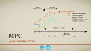
14. PREDICTIVE CONTROL WITHIN ONE
OPTIMIZATION WINDOW
• Current Time: ki
• Prediction horizon (Np): Number of prediction samples
• Control horizon (Nc): dictating number of parameters used to capture the
future control trajectory
14Model Predictive Control/Dec 2016/University of Tehran/School of Mechanical Engineering

15. PREDICTIVE CONTROL WITHIN ONE
OPTIMIZATION WINDOW
15Model Predictive Control/Dec 2016/University of Tehran/School of Mechanical Engineering

16. PREDICTION OF STATE AND OUTPUT VARIABLES
x(ki + 1 | ki) = Ax(ki) + BΔu(ki)
x(ki + 2 | ki) = Ax(ki+1|ki) + BΔu(ki+1)
= A2x(ki) + ABΔu(ki) + BΔu(ki+1)
⋮ ⋮
x(ki + Np | ki) = ANpx(ki) + ANp-1BΔu(ki) + ANp-2BΔu(ki+1)+...
+ ANp-NcBΔu(ki+Nc-1)
16Model Predictive Control/Dec 2016/University of Tehran/School of Mechanical Engineering

17. PREDICTION OF STATE AND OUTPUT VARIABLES
y(ki+1|ki) = CAx(ki) + CBΔu(ki)
y(ki+2|ki) = CA2x(ki) + CABΔu(ki) + CBΔu(ki+1)
⋮ ⋮
y(ki+Np|ki) = CANpx(ki) + CANp-1BΔu(ki) + CANp-2BΔu(ki+1)+
. . . + CANp-NcBΔu(ki+Nc-1)
17Model Predictive Control/Dec 2016/University of Tehran/School of Mechanical Engineering

18. PREDICTION OF STATE AND OUTPUT VARIABLES
𝑌 =
𝑦(𝑘𝑖 + 1|𝑘𝑖)
𝑦(𝑘𝑖 + 2|𝑘𝑖)
𝑦(𝑘𝑖 + 3|𝑘𝑖)
⋮
𝑦(𝑘𝑖 + 𝑁 𝑝|𝑘𝑖)
, 𝑈 =
𝛥𝑢(𝑘𝑖)
𝛥𝑢(𝑘𝑖 + 1)
𝛥𝑢(𝑘𝑖 + 2)
⋮
𝛥𝑢(𝑘𝑖 + 𝑁𝑐 − 1)
18Model Predictive Control/Dec 2016/University of Tehran/School of Mechanical Engineering

19. PREDICTION OF STATE AND OUTPUT VARIABLES
19Model Predictive Control/Dec 2016/University of Tehran/School of Mechanical Engineering

20. OPTIMIZATION
Cost function
𝑅 𝑠 = 𝑜𝑛𝑒𝑠 𝑁 𝑝 ,
1 ∗ 𝑟 𝑘𝑖 = 𝑅 𝑠 𝑟 𝑘𝑖
𝑅 = 𝑟 𝜔 𝐼 𝑁 𝑐×𝑁𝑐 (𝑟 𝜔 ≥ 0)
20Model Predictive Control/Dec 2016/University of Tehran/School of Mechanical Engineering
• First term is linked to the objective of minimizing the errors between
the predicted output and the set-point signal.
• Second term reflects the consideration given to impact of ΔU when the
objective function J is made to be as small as possible.

21. OPTIMIZATION
Hessian matrix
21Model Predictive Control/Dec 2016/University of Tehran/School of Mechanical Engineering

22. MATLAB EXAMPLE 2
22Model Predictive Control/Dec 2016/University of Tehran/School of Mechanical Engineering

23. CLOSED-LOOP CONTROL SYSTEM
23Model Predictive Control/Dec 2016/University of Tehran/School of Mechanical Engineering

24. BLOCK DIAGRAM OF DISCRETE-TIME PREDICTIVE
CONTROL SYSTEM
24Model Predictive Control/Dec 2016/University of Tehran/School of Mechanical Engineering

25. STATE ESTIMATE PREDICTIVE CONTROL
25Model Predictive Control/Dec 2016/University of Tehran/School of Mechanical Engineering

26. MPC DESIGN WITH CONSTRAINTS
26Model Predictive Control/Dec 2016/University of Tehran/School of Mechanical Engineering
With sampling interval Δt = 0.1

27. MPC DESIGN WITH CONSTRAINTS
27Model Predictive Control/Dec 2016/University of Tehran/School of Mechanical Engineering
The prediction horizon Np = 10 and the control horizon Nc = 3. There is
no weight on the control signal, i.e., 𝑅 = 0. Examine what happens if the
control amplitude is limited to ±25 by saturation.

28. MPC DESIGN WITH CONSTRAINTS
CASE A. WITHOUT CONTROL SATURATION
28Model Predictive Control/Dec 2016/University of Tehran/School of Mechanical Engineering

29. MPC DESIGN WITH CONSTRAINTS
CASE B. WITH CONTROL SATURATION
29Model Predictive Control/Dec 2016/University of Tehran/School of Mechanical Engineering

30. MPC DESIGN WITH CONSTRAINTS
CASE C. WITH MODIFIED CONTROL SATURATION
30Model Predictive Control/Dec 2016/University of Tehran/School of Mechanical Engineering

31. MPC DESIGN WITH CONSTRAINTS
CASE C. WITH MODIFIED CONTROL SATURATION
31Model Predictive Control/Dec 2016/University of Tehran/School of Mechanical Engineering

32. MPC DESIGN WITH CONSTRAINTS
CASE COMPARISON
32Model Predictive Control/Dec 2016/University of Tehran/School of Mechanical Engineering

33. FREQUENTLY USED OPERATIONAL CONSTRAINTS
Control Variable Incremental Variation
• These are hard constraints on the size of the control signal movements, i.e., on the
rate of change of the control variables (Δu(k))
Amplitude of the Control Variable
• These are the most commonly encountered constraints among all constraint types.
• These are the physical hard constraints on the system.
Output Constraints
• Output constraints are often implemented as ‘soft’ constraints.
• Output constraints often cause large changes in both the control and incremental
control variables when they are enforced.
Model Predictive Control/Dec 2016/University of Tehran/School of Mechanical Engineering 33

34. NUMERICAL SOLUTIONS USING QUADRATIC
PROGRAMMING
Model Predictive Control/Dec 2016/University of Tehran/School of Mechanical Engineering 34
Quadratic
Programming
Inequality
Constraints
Equality
Constraints

35. QUADRATIC PROGRAMMING FOR EQUALITY CONSTRAINTS
Model Predictive Control/Dec 2016/University of Tehran/School of Mechanical Engineering 35

36. QUADRATIC PROGRAMMING FOR EQUALITY CONSTRAINTS
Model Predictive Control/Dec 2016/University of Tehran/School of Mechanical Engineering 36
𝑥1 = 0.5 → 𝑥2 = 1 − 𝑥1 = 0.5

37. LAGRANGE MULTIPLIERS
Model Predictive Control/Dec 2016/University of Tehran/School of Mechanical Engineering 37
Constraint equation: 𝑀𝑥 = 𝛾
The procedure of minimization is to take the first partial derivatives with
respect to the vectors x and λ, and then equate these derivatives to zero:

38. LAGRANGE MULTIPLIERS
EXAMPLE
Model Predictive Control/Dec 2016/University of Tehran/School of Mechanical Engineering 38

39. LAGRANGE MULTIPLIERS
EXAMPLE
Model Predictive Control/Dec 2016/University of Tehran/School of Mechanical Engineering 39

40. ACTIVE SET METHOD
Model Predictive Control/Dec 2016/University of Tehran/School of Mechanical Engineering 40
λi ≥ 0
λi < 0
The point is a local solution
The objective function value can
be decreased by relaxing the
constraint i

41. Model Predictive Control/Dec 2016/University of Tehran/School of Mechanical Engineering 41
MINIMIZATION WITH INEQUALITY CONSTRAINTS
EXAMPLE

42. Model Predictive Control/Dec 2016/University of Tehran/School of Mechanical Engineering 42
Clearly the third element in λ is negative, therefore, the third constraint is an
inactive constraint and will be dropped from the constrained equation
λ =
5
3
→ x =
0.3333
1.3333
−0.6667
MINIMIZATION WITH INEQUALITY CONSTRAINTS
EXAMPLE
Inactive
constraint
Inactive
constraint

43. REFERENCES
1. Model Predictive Control System Design and
Implementation Using MATLAB, Liuping
Wang
2. Model Predictive Control, 2nd edition, E.F.
Camacho
3. A Lecture on Model Predictive Control, Jay
H. Lee
4. Model Predictive Control: Basic Concepts, A.
Bemporad
5. Lecture 14 - Model Predictive Control Part
1: The Concept, Gorinevsky
6. Principles of Optimal Control, Lecture 16
Model Predictive Control
7. Model Predictive Control, 4 Lectures 2016,
Mark Cannon
8. Model Predictive Control, S. Boyd

44. PRESENTED BYThanks for your
attention! Pooyan Nayyeri
Faraz AbedAzad
Model Predictive Control/Dec 2016/University of Tehran/School of Mechanical Engineering 44