Download to read offline
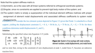
![which can be expressed in matrix
form as
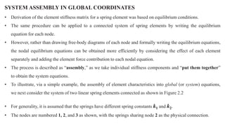
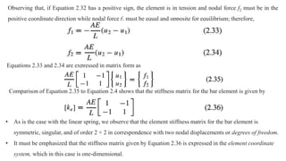
• [ke] is defined as the element stiffness matrix in the element coordinate system (or local system), {u} is the
column matrix (vector) of nodal displacements, and {f} is the column matrix (vector) of element nodal
forces.
• A general matrix is designated by brackets [ ] and a column matrix (vector) by braces { }.
• Equation 2.6 shows that the element stiffness matrix for the linear spring element is a 2 × 2 matrix.
• This corresponds to the fact that the element exhibits two nodal displacements and that the two displacements
are not independent (that is, the body is continuous and elastic).
• Furthermore, the matrix is symmetric.](https://image.slidesharecdn.com/femchapter2-211118115503/85/Finite-element-method-6-320.jpg)
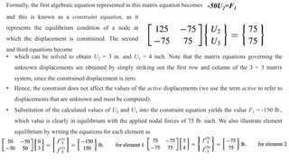
![• A symmetric matrix has off-diagonal terms such that kij = kji. Symmetry of the stiffness matrix is indicative of
the fact that the body is linearly elastic and each displacement is related to the other by the same physical
phenomenon.
• For example, if a force F (positive, tensile) is applied at node 2 with node 1 held fixed, the relative displacement
of the two nodes is the same as if the force is applied symmetrically (negative, tensile) at node 1 with node 2
fixed.
• As will be seen as more complicated structural elements are developed, this is a general result: An element
exhibiting N degrees of freedom has a corresponding N × N, symmetric stiffness matrix.
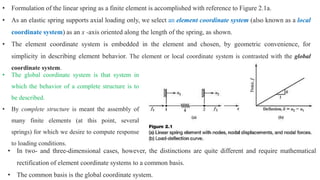
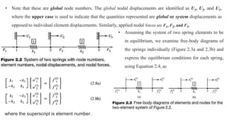
• Next consider solution of the system of equations represented by Equation 2.4.
• In general, the nodal forces are prescribed and the objective is to solve for the unknown nodal displacements.
Formally, the solution is represented by
where [ke]-1 is the inverse of the element stiffness matrix.](https://image.slidesharecdn.com/femchapter2-211118115503/85/Finite-element-method-7-320.jpg)
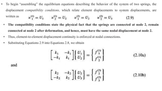
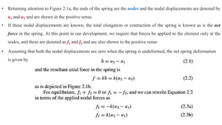
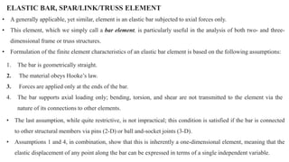
![Next, we refer to the free-body diagrams of each of the three nodes. The equilibrium conditions for nodes 1, 2, and
3 show that
Substituting into Equation 2.13, we obtain the final result:
which is of the form [K]{U} = {F}, similar to Equation 2.5.
However, Equation 2.15 represents the equations governing the system composed of two connected spring
elements. By direct consideration of the equilibrium conditions, we obtain the system stiffness matrix [K] (note
use of upper case) as
respectively.](https://image.slidesharecdn.com/femchapter2-211118115503/85/Finite-element-method-12-320.jpg)
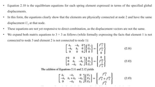
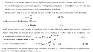
![As we have two conditions that must be satisfied by each of two one-dimensional functions, the simplest
forms for the interpolation functions are polynomial forms:
where the polynomial coefficients are to be determined via satisfaction of the boundary (nodal) conditions.
Application of conditions represented by Equation 2.19 yields a0 = 1, b0 = 0 while
Equation 2.20 results in a1 = -(1/L) and b1 = x/L . Therefore, the interpolation functions are
and the continuous displacement function is represented by the discretization
As will be found most convenient subsequently, Equation 2.25 can be expressed in matrix form as
where [N ] is the row matrix of interpolation functions and {u} is the column matrix (vector) of nodal
displacements.](https://image.slidesharecdn.com/femchapter2-211118115503/85/Finite-element-method-19-320.jpg)


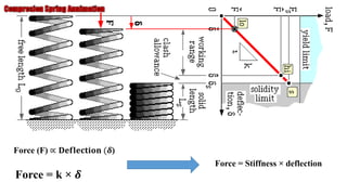
This document provides an introduction to finite element analysis and stiffness matrices. It discusses modeling a linear spring and elastic bar as finite elements. The key points are: 1. The stiffness matrix contains information about an element's resistance to deformation from applied loads. It relates nodal displacements and forces for the element. 2. A linear spring and elastic bar can each be modeled as a finite element with a 2x2 stiffness matrix. Their matrices are derived from relating nodal displacements to forces based on Hooke's law and the element's geometry. 3. A system of multiple elements is modeled by assembling the individual element stiffness matrices into a global system stiffness matrix, relating total nodal displacements and forces