Download to read offline
![Basic Steps in the Finite Element Method
Time Independent Problems
- Domain Discretization
- Select Element Type (Shape and Approximation)
- Derive Element Equations (Variational and Energy Methods)
- Assemble Element Equations to Form Global System
[K]{U} = {F}
[K] = Stiffness or Property Matrix
{U} = Nodal Displacement Vector
{F} = Nodal Force Vector
- Incorporate Boundary and Initial Conditions
- Solve Assembled System of Equations for Unknown Nodal
Displacements and Secondary Unknowns of Stress and Strain Values](https://image.slidesharecdn.com/femlecture-220106173146/85/Fem-lecture-10-320.jpg)
![Simple Element Equation Example
Direct Stiffness Derivation
1 2
k
u1 u2
F1 F2
}
{
}
]{
[
rm
Matrix Fo
in
or
2
Node
at
m
Equilibriu
1
Node
at
m
Equilibriu
2
1
2
1
2
1
2
2
1
1
F
u
K
F
F
u
u
k
k
k
k
ku
ku
F
ku
ku
F
Stiffness Matrix Nodal Force Vector](https://image.slidesharecdn.com/femlecture-220106173146/85/Fem-lecture-17-320.jpg)
![One-Dimensional Bar Element
udV
f
u
P
u
P
edV j
j
i
i
}
]{
[
:
Law
Strain
-
Stress
}
]{
[
}
{
]
[
)
(
:
Strain
}
{
]
[
)
(
:
ion
Approximat
d
B
d
B
d
N
d
N
E
Ee
dx
d
u
x
dx
d
dx
du
e
u
x
u
k
k
k
k
k
k
L
T
T
j
i
T
L
T
T
fdx
A
P
P
dx
E
A
0
0
]
[
}
{
}
{
}
{
]
[
]
[
}
{ N
δd
δd
d
B
B
δd
L
T
L
T
fdx
A
dx
E
A
0
0
]
[
}
{
}
{
]
[
]
[ N
P
d
B
B
Vector
ent
Displacem
Nodal
}
{
Vector
Loading
]
[
}
{
Matrix
Stiffness
]
[
]
[
]
[
0
0
j
i
L
T
j
i
L
T
u
u
fdx
A
P
P
dx
E
A
K
d
N
F
B
B
}
{
}
]{
[ F
d
K ](https://image.slidesharecdn.com/femlecture-220106173146/85/Fem-lecture-19-320.jpg)

![Linear Approximation Scheme
Vector
ent
Displacem
Nodal
}
{
Matrix
Function
ion
Approximat
]
[
}
]{
[
1
)
(
)
(
1
2
1
2
1
2
1
2
2
1
1
2
1
1
2
1
2
1
2
1
1
2
1
d
N
d
N
nt
Displaceme
Elastic
e
Approximat
u
u
L
x
L
x
u
u
u
u
x
u
x
u
L
x
u
L
x
x
L
u
u
u
u
L
a
a
u
a
u
x
a
a
u
x (local coordinate system)
(1) (2)
i
u j
u
L
x
(1) (2)
u(x)
x
(1) (2)
1(x) 2(x)
1
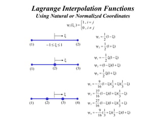
k(x) – Lagrange Interpolation Functions](https://image.slidesharecdn.com/femlecture-220106173146/85/Fem-lecture-21-320.jpg)
![Element Equation
Linear Approximation Scheme, Constant Properties
Vector
ent
Displacem
Nodal
}
{
1
1
2
]
[
}
{
1
1
1
1
1
1
1
1
]
[
]
[
]
[
]
[
]
[
2
1
2
1
0
2
1
0
2
1
0
0
u
u
L
Af
P
P
dx
L
x
L
x
Af
P
P
fdx
A
P
P
L
AE
L
L
L
L
L
AE
dx
AE
dx
E
A
K
o
L
o
L
T
L
T
L
T
d
N
F
B
B
B
B
1
1
2
1
1
1
1
}
{
}
]{
[
2
1
2
1 L
Af
P
P
u
u
L
AE o
F
d
K](https://image.slidesharecdn.com/femlecture-220106173146/85/Fem-lecture-22-320.jpg)
![Quadratic Approximation Scheme
}
]{
[
)
(
)
(
)
(
4
2
3
2
1
3
2
1
3
3
2
2
1
1
2
3
2
1
3
2
3
2
1
2
1
1
2
3
2
1
d
N
nt
Displaceme
Elastic
e
Approximat
u
u
u
u
u
x
u
x
u
x
u
L
a
L
a
a
u
L
a
L
a
a
u
a
u
x
a
x
a
a
u
x
(1) (3)
1
u 3
u
(2)
2
u
L
u(x)
x
(1) (3)
(2)
x
(1) (3)
(2)
1
1(x) 3(x)
2(x)
3
2
1
3
2
1
7
8
1
8
16
8
1
8
7
3
F
F
F
u
u
u
L
AE
Equation
Element](https://image.slidesharecdn.com/femlecture-220106173146/85/Fem-lecture-23-320.jpg)
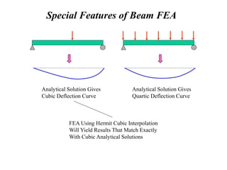
![One-Dimensional Beam Element
Deflection of an Elastic Beam
2
2
4
2
3
1
1
2
1
1
2
2
2
4
2
2
2
3
1
2
2
2
1
2
2
1
,
,
,
,
,
dx
dw
u
w
u
dx
dw
u
w
u
dx
w
d
EI
Q
dx
w
d
EI
dx
d
Q
dx
w
d
EI
Q
dx
w
d
EI
dx
d
Q
q
q
I = Section Moment of Inertia
E = Elastic Modulus
f(x) = Distributed Loading
(1) (2)
Typical Beam Element
1
w
L
2
w
1
q 2
q
1
M 2
M
1
V 2
V
x
Virtual Strain Energy = Virtual Work Done by Surface and Body Forces
wdV
f
w
Q
u
Q
u
Q
u
Q
edV 4
4
3
3
2
2
1
1
L
T
L
dV
f
w
Q
u
Q
u
Q
u
Q
dx
EI
0
4
4
3
3
2
2
1
1
0
]
[
}
{
]
[
]
[ N
d
B
B T
(Four Degrees of Freedom)](https://image.slidesharecdn.com/femlecture-220106173146/85/Fem-lecture-27-320.jpg)
![Beam Element Equation
L
T
L
dV
f
w
Q
u
Q
u
Q
u
Q
dx
EI
0
4
4
3
3
2
2
1
1
0
]
[
}
{
]
[
]
[ N
d
B
B T
4
3
2
1
}
{
u
u
u
u
d ]
[
]
[
]
[ 4
3
2
1
dx
d
dx
d
dx
d
dx
d
dx
d f
f
f
f
N
B
2
2
2
2
3
0
2
3
3
3
6
3
6
3
2
3
3
6
3
6
2
]
[
]
[
]
[
L
L
L
L
L
L
L
L
L
L
L
L
L
EI
dx
EI
L
B
B
K T
L
L
fL
Q
Q
Q
Q
u
u
u
u
L
L
L
L
L
L
L
L
L
L
L
L
L
EI
6
6
12
2
3
3
3
6
3
6
3
2
3
3
6
3
6
2
4
3
2
1
4
3
2
1
2
2
2
2
3
f
f
f
f
L
L
fL
dx
f
dx
f
L
L
T
6
6
12
]
[
0
4
3
2
1
0
N](https://image.slidesharecdn.com/femlecture-220106173146/85/Fem-lecture-29-320.jpg)

The document provides an introduction to finite element methods. It discusses how finite element analysis (FEA) is used to solve engineering and science problems involving complex geometries and conditions. FEA works by dividing a body into finite elements and approximating variable fields within each element. This discretization process sets up algebraic equations that approximate the continuous solution. FEA can model problems with complex shapes, loads, materials and include time-dependent effects. It has advantages over closed-form solutions and its accuracy can be improved by refining the mesh. Examples of 1D and 2D elements and approximations are presented.