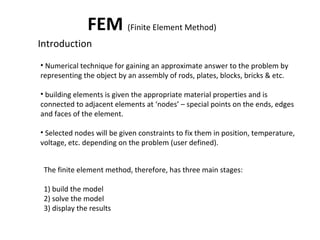
Finite element analysis (FEA) is a numerical technique used to approximate solutions to boundary value problems by dividing the domain into smaller elements. The document discusses the three main stages of FEA: building the model, solving the model, and displaying the results. It provides details on how to create nodes and finite elements to represent an object's geometry, assign material properties and constraints, define the type of analysis, and select parameters to display in the results. Examples of different types of FEA analyses are also listed, such as static, thermal, modal, and buckling analyses.

1. introduction to
FEA software
finite element analysis

2. FEM (Finite Element Method)
Introduction
• Numerical technique for gaining an approximate answer to the problem by
representing the object by an assembly of rods, plates, blocks, bricks & etc.
• building elements is given the appropriate material properties and is
connected to adjacent elements at ‘nodes’ – special points on the ends, edges
and faces of the element.
• Selected nodes will be given constraints to fix them in position, temperature,
voltage, etc. depending on the problem (user defined).
The finite element method, therefore, has three main stages:
1) build the model
2) solve the model
3) display the results

3. Build the model
• create nodes in positions to represent the object’s shape or import from an existing
CAD model
• refine as required.
• create finite elements (beams, plates, bricks, etc) between the nodes
• assign material properties to the elements
• assign constraints to selected nodes
• assign applied forces to the appropriate nodes.
Solve the model
•define the type of analysis you want e.g. static linear, vibrational modes, dynamic
response with time, etc.
Display the results
• select which parameters you want to display e.g. displacement, principal stress,
temperature, voltage,
• display as 2D or 3D contour plots, and/or as tables of numerical values, before
inferring anything from the results, they must first be validated,
• validation requires confirming mesh convergence has occurred and that values are in
line with expectations from hand calculations, experiments or past experience,
• mesh convergence requires refining the mesh repeatedly and solving until the
results
no longer change appreciably.

4. The Work
Flow
1.1 Mesh
• A finite element mesh consists of nodes (points) and elements (shapes which link the nodes
together).
• Elements represent material so they should fill the volume of the object being modeled.
1.2 Analysis
• Global properties such as analysis type, physical constants, solver settings and output options
by editing the Analysis item in the outline tree
1.3 Geometry
If you generate a mesh from a STEP or IGES file exported from CAD then these files are shown in
the Geometry group. Each geometry item can be auto-meshed to generate a mesh.
1.4 Components & Materials
• A component is an exclusive collection of elements. Every element must belong to exactly one
component. The default component is created automatically and cannot be deleted.
• Each component containing some elements must have a material assigned to it. The same
material can be shared between several components.
1.5 Named Selections
• A named selection is a non-exclusive collection of nodes, elements or faces.
• Named selections are used for applying loads and constraints.
1.6 Loads & Constraints
• This group contains all the loads and constraints in the model. It can also contain load cases
with their own loads.
1.7 Solution
After solving, the results are shown under the Solution branch in the outline tree. You can click
on a field value to display a colored contour plot of it.

5. GUI graphic user interface
• the toolbars at the top, arranged into model-building tools and the graphics display options.
• the model structure and solution displayed in an outline tree in the left panel
• a graphic display area of the model
1.2.1_basic_graphics_tutorial.liml

6. Modelling
• uses only nodes and elements
• imported CAD models in stp & iges format
• model is a mesh of elements. Each element has nodes which are simply points on
the element. Elements can only be connected to other elements node-to-node.
• Elements themselves have very simple shapes like lines, triangles, squares, cubes
and pyramids.
Each element is formulated to obey a particular law of science. For example:
• static analysis - the elements are formulated to relate displacement and stress according to the
theory of mechanics of materials.
• modal vibration - the elements are formulated to obey deflection shapes and frequencies
according to the theory of structural dynamics.
• thermal analysis - the elements relate temperature and heat according to heat transfer theory.

7. • Always begin a manual mesh by
creating a coarse mesh; it can always be
refined later.
• finite elements are 3D. The elements
that appear flat and 2D do actually have
the third dimension, of thickness.
• 3D Elements usually be created from a
2D flat shape. This initial 2D mesh can
be created either by a combination of
nodes and elements or by using readymade template patterns.
• Editing tools are available for
modifying the 2Dmesh. Once the coarse
mesh is complete, whether it be 2D or
3D in appearance, it will need to be
refined before running the Solver.

8. Meshing Tools
creating tools, that bring into existence
a two dimensional mesh
editing tools, that form and modify the created 2D mesh
tools that will convert the two dimensional mesh
into 3D meshes
refinement tools for converging results

9. Geometric Model
1
1
11
Element Properties:
Mesh size: 11 x 4x 2
Young Modulus: 200e9 N/m2
Poisson ratio: 0.3
Density: 7860 kg/m3
2
All dimension in m unless stated otherwise

10. Analysis Types
Warning:
!
The finite element method uses a mathematical formulation of physical theory to represent physical
behavior. Assumptions and limitations of theory (like beam theory, plate theory, Fourier theory, etc.) must
not be violated by what we ask the software to do. A competent user must have a good physical grasp of the
problem so that errors in computed results can be detected and a judgment made as to whether the results
are to be trusted or not. Please validate your results!
• FEA follows the law of 'Garbage in, Garbage out'.
The choice of element type, mesh layout, correctness of applied constraints will directly affect the stability
and accuracy of the solution.
Tips:
The outline tree presents all the information needed about your
model and allows you to perform various actions on the model itself.
You will always begin at the top, changing the analysis type if you do
not want the default, 3D static analysis.
Items that appear in red indicate missing or erroneous information, so right
click them for a What's wrong? clue.

11. Analysis Types
Tips:
Apply your loads and constraints to element faces rather than nodes. Mesh refinements will automatically
transfer element face loads and constraints to the newly created elements, whereas loads and constraints
applied to nodes are not automatically transferred to the new Elements.

12. Analysis Types - examples
• Static analysis of a pressurized cylinder
• Thermal analysis of a plate being cooled
• Modal vibration of a cantilever beam
• Dynamic response of a crane frame
• Magnetostatic analysis of a current carrying wire
• DC circuit analysis
• Electrostatic analysis of a capacitor
• Acoustic analysis of an organ pipe
• Buckling of a column
• Fluid flow around a cylinder

13. Static analysis of a pressurized cylinder
A cylinder of 2m radius, 10m length, 0.2m thickness, Young's modulus 200e9 N/m2 and Poisson ratio 0.285 will be analyzed to
determine its hoop stress caused by an internal pressure of 100N. From shell theory, the circumferential or hoop stress for a thin
cylinder of constant radius and uniform internal pressure is given by :
σ = (pressure × radius) / thickness
σ = (100 × 2) / 0.2
σ = 1000 N/m2

14. Static analysis of a pressurized cylinder
A cylinder of 2m radius, 10m length, 0.2m thickness, Young's modulus 200e9 N/m2 and Poisson ratio 0.285 will be analyzed to
determine its hoop stress caused by an internal pressure of 100N. From shell theory, the circumferential or hoop stress for a thin
cylinder of constant radius and uniform internal pressure is given by :
σ = (pressure × radius) / thickness
σ = (100 × 2) / 0.2
σ = 1000 N/m2

15. Thermal analysis of a plate being cooled
A plate of cross-section thickness 0.1m at an initial temperature of 250°C is suddenly immersed in an oil bath of temperature
50°C. The material has a thermal conductivity of 204W/m/°C, heat transfer coefficient of 80W/m2/°C, density 2707 kg/m3 and
a specific heat of 896 J/kg/°C. It is required to determine the time taken for the slab to cool to a temperature of 200*C.
For Biot numbers less than 0.1, the temperature anywhere in the cross-section will be the same with time.
Bi = hL/k = (80)(0.1)/(204) = 0.0392
From classical heat transfer theory the following lumped analysis heat transfer formula can be used.
(T(t)-Ta)/(To-Ta) = e-(mt)
Ta = temperature of oil bath, To = initial temperature
where m = h/ ρ Cp(L/2), h = heat transfer coefficient
ρ = density, Cp = specific heat, L = thickness
m = 80/[(2707)(896)(0.1/2)]
m = 1/1515.92 s-1
(200 - 50) / (250 - 50) = e(-t/1515.92)
t = ln (4) X 1515.92
t = 436 s

16. Modal vibration of a cantilever beam
A cantilever beam of length 1.2m, cross-section 0.2m × 0.05m, Young's modulus 200×10 9 Pa, Poisson
ratio 0.3 and density 7860 kg/m3. The lowest natural frequency of this beam is required to be
determined.
For thin beams, the following analytical equation is used to calculate the first natural frequency :
f = (3.52/2π)[(k / 3 × M)]1/2
f = frequency, M = mass
M = density × volume
M = 7860 × 1.2 × 0.05 × 0.2
M = 94.32 kg
k = spring stiffness
k = 3×E×I / L3
I = moment of inertia of the cross-section.
E = Young's modulus, L = beam length
I = (1/12)(bh3)
I = (1/12) (0.2 x 0.053)
I = 2.083×10-6 m4
k = (3 × 200×109 × 2.083×10-6) / 1.23
k = 723.379×103 N/m
f = (3.52/2 × 3.14) [(723.379×103/ 3 × 94.32)]1/2
f = 28.32 Hz
Beginners guide:pg 42

17. Dynamic response of a crane frame
Beginners guide:pg 46

18. Buckling of a column
The eigen value buckling of a column with a fixed end will be solved. The column has a length of 100mm, a
square cross-section of 10mm and Young's modulus 200000 N/mm2 .
The critical load for a fixed end Euler column is π2EI/(4L2)
E = Young's modulus, I = moment of inertia
I = 104/12 = 833.33mm4
L = length
Critical load = π2 200000 × 833.33 / (4×1002)= 41123.19 N
Beginners guide:pg 76

19. Fluid flow around a cylinder
A confined streamlined flow around a cylinder will be analyzed for the flow potentials and velocity
distributions around the cylinder. The inward flow velocity is 1 m/s . The ambient pressure is 1×10 5 Pa,
density 1000 kg/m3 .

20. Modeling Errors
Results can only be as accurate as your model. Use rough estimates from hand calculations, experiment or
experience to check whether or not the results are reasonable. If the results are not as expected, your model
may have serious errors which need to be identified.
Too coarse a mesh
• the narrower the rectangles, the more
accurate will be the result.
• Concentrate the mesh refinement in those
areas where the accuracy can be improved,
while leaving unchanged those areas that
are already accurate.
• Run at least one model to identify the
areas where the values are changing a lot
and the areas where values are remaining
more or less the same. The second run will
be the refined model.

21. Modeling Errors
Wrong choice of elements
• Plate-like geometries such as walls, where the thickness is less in comparison to its other dimensions,
should be modeled with either shell elements or quadratic solid elements .
• Shell, beam and membrane elements should not be used where their simplified assumptions do not apply.
For example beams that are too thick, membranes that are too thick for plane stress and too thin
for plane strain, or shells
Linear elements
Linear elements (elements with no mid-side nodes) are too stiff in
bending so they typically have to be refined more than quadratic
elements (elements with mid-side nodes) for results to converge.
4.5.4 Severely distorted elements
Element shapes that are compact and regular give the greatest accuracy. The ideal triangle is
equilateral, the ideal quadrilateral is square, the ideal hexahedron is a cube of equal side length, etc.
Distortions tend to reduce accuracy by making the element stiffer than it would be otherwise, usually
degrading stresses more than displacements.
Shape distortions will occur in FE modeling because it is quite impossible to represent structural geometry
with perfectly shaped elements. Any deterioration in accuracy will only be in the vicinity of the badly shaped
elements and will not propagate through the model (St. Venant's principle).
These artificial disturbances in the field values should not be erroneously accepted as actually being
present.

22. Modeling Errors
Severely distorted elements
• Element shapes that are compact and regular give the greatest accuracy. The ideal triangle is equilateral,
the ideal quadrilateral is square, the ideal hexahedron is a cube of equal side length, etc.
• Distortions tend to reduce accuracy by making the element stiffer than it would be otherwise, usually
degrading stresses more than displacements.
• Shape distortions will occur in FE modeling because it is quite impossible to represent structural geometry
with perfectly shaped elements. Any deterioration in accuracy will only be in the vicinity of the badly shaped
elements and will not propagate through the model (St. Venant's principle).
These artificial disturbances in the field values should not be erroneously accepted as actually being
present.
Avoid large aspect ratios. A length to breadth
ratio of generally not more than 3.
Avoid strongly curved sides in quadratic
elements.
Highly skewed. A skewed angle of generally
not more than 30 degrees.
Off center mid-side nodes.
A quadrilateral should not look almost like a
triangle.

23. Modeling Errors
Mesh discontinuities
• Element sizes should not change abruptly from fine to coarse.
Rather they should make the transition gradually.
• Nodes cannot be connected to element
edges. Such arrangements will result in
gaps and penetrations that do not occur in
reality.
• Corner nodes of quadratic elements
should not be connected to mid-side
nodes. Although both edges deform
quadratically, they are not deflecting in
sync with each other.
• Linear elements (no mid-side node) should not be connected to the
midside nodes of quadratic elements, because the edge of the
quadratic element deforms quadratically whereas the edges of the
linear element deform linearly.
• Avoid using linear elements with quadratic elements as the mid side node
will open a gap or penetrate the linear element.

24. Modeling Errors
Non-linearities
• Some FEA software can model only the linear portion
of the stress-strain curve and large deformations where
the stiffness or load changes with deformation.
• Shell elements under bending loads should not deform
by more than half their thickness otherwise
non-linear membrane action occurs in the real world to
resist further bending.
Improper constraints
Fixed supports will result in less deformation that simple supports which permit material to move within
the plane of support.
Rigid body motion
In static analysis, for a structure to be stressed all rigid body motion must be eliminated. For 2D problems there
are two translational (along the X- & Y-axes) and one rotational (about the Z-axis) rigid body motions. For 3D
problems there are three translational (along the X-, Y- & Z-axes) and three rotational (about the X-,Y- & Z-axes)
rigid body motions. Rigid body motion can be eliminated by applying constraints such as fixed support,
displacement and rotx, roty and rotz.