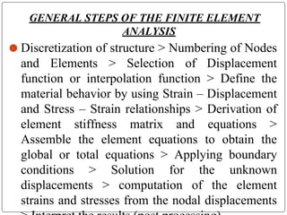
This document outlines the objectives, course outcomes, and units covered in a finite element analysis course. The objective is to equip students with fundamentals of FEA and introduce the steps involved in discretization, applying boundary conditions, assembling stiffness matrices, and solving problems. The course covers basic FEA concepts, one-dimensional elements, two-dimensional elements, axisymmetric problems, isoparametric elements, and dynamic analysis. Students will learn to formulate and solve structural and heat transfer problems using various finite elements.
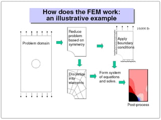
Here are the steps to solve this problem using Galerkin's technique:
1. Write the weak form of the differential equation:
∫(AEδu - δu d2u/dx2 - aδux)dx = 0
2. Choose the trial function u(x) = a0 + a1x
3. Choose the weight function δu = 1, x, x2...
4. Substitute the trial function and weight functions into the weak form and integrate by parts.
5. Apply the essential boundary conditions to eliminate terms involving du/dx at boundaries.
6. Solve the resulting algebraic equations to determine the unknown coefficients a0 and a1
This document outlines the course objectives and contents for a finite element methods in mechanical design course. The key points are:
1. The course will introduce mathematical modeling concepts and teach how to apply finite element methods (FEM) to solve a range of engineering problems.
2. The content will cover one-dimensional, two-dimensional, and three-dimensional FEM analysis. Solution techniques like inversion methods and dynamic analysis will also be discussed.
3. Applications of FEM include stress analysis, buckling analysis, vibration analysis, heat transfer analysis, and fluid flow analysis for both structural and non-structural problems.
This document outlines a Computer Aided Engineering course for third year mechanical engineering students. The course objectives are to understand CAE concepts and finite element analysis, learn discretization and meshing techniques, apply FEM to solve mechanics problems, and study applications in domains like computational fluid dynamics, injection molding, and manufacturing simulations. The syllabus covers elemental properties, meshing, 1D and 2D finite element analysis, nonlinear and dynamic analysis, and applications. References include textbooks and online courses on finite element basics, advanced analysis, and ANSYS tutorials.
This document discusses the finite element method (FEM) for numerical analysis of engineering problems. It describes the general steps of FEM which include discretizing the domain into simple geometric elements, choosing interpolation functions, deriving the element stiffness matrices, assembling the matrices into a global system, applying boundary conditions, and solving for displacements/stresses. FEM allows for approximate solutions of complex problems involving various material properties, geometries, and loading conditions.
Introduction of Finite Element AnalysisMuthukumar V
This document discusses the finite element method (FEM) for numerical analysis of engineering problems. It describes the general steps of FEM which include discretizing the domain into simple geometric elements, choosing interpolation functions, deriving the element stiffness matrices, assembling the system to solve for displacements, and computing stresses and strains. FEM can be used to solve structural and non-structural problems and overcomes limitations of experimental and analytical methods for complex systems. The key aspects are subdividing the domain, selecting interpolation functions, deriving element equations, assembling the global system, applying boundary conditions, and solving for unknowns.
Topics to be discussed-
Introduction
How Does FEM Works?
Types Of Engineering Analysis
Uses of FEM in different fields
How can the FEM Help the Design Engineer?
How can the FEM Help the Design Organization?
Basic Steps & Phases Involved In FEM
Advantages and disadvantages
The Future Scope
References.
The document provides an introduction to the finite element method (FEM). It discusses how FEM can be used to obtain approximate solutions to boundary value problems in engineering. It outlines the general steps involved, including preprocessing (defining the model), solution/processing (computing unknown values), and postprocessing (analyzing results). Examples of FEM applications include structural analysis, fluid flow, heat transfer, and more. The key aspects of FEM include discretizing the domain into simple elements, choosing shape functions to approximate variations within each element, and assembling the element equations into a global system of equations to solve.
*Need of finite element analysis
*Introduction to approaches used in Finite Element Analysis such as direct approach and energy approach
*Boundary conditions: Types
*Rayleigh-Ritz Method
*Galerkin Method
This document describes a case study analyzing the maximum deflection of a cantilever beam using finite element analysis software ANSYS. It first provides background on finite element analysis and its general steps. It then outlines the specific steps taken in ANSYS to model and analyze a cantilever beam with an end load, including preprocessing, solution, and postprocessing stages. The results found the maximum deflection to be 0.73648m and the von-mises stress to be 286.19 N/m. The document concludes with thanks for reading.
This document discusses the finite element method (FEM) for engineering analysis. It explains that FEM involves discretizing a continuous structure into smaller, finite elements and then solving the equations for each element. The general steps of FEM are: 1) discretizing the structure into elements connected at nodes, 2) numbering nodes and elements, 3) selecting displacement functions, 4) defining material behavior, 5) deriving element stiffness matrices, 6) assembling equations, 7) applying boundary conditions, 8) solving for displacements, 9) computing strains and stresses, and 10) interpreting results. Discretization is the process of subdividing a structure into smaller finite elements that are then assembled to represent the original structure.
This document discusses the finite element method (FEM) for engineering analysis. It explains that FEM involves discretizing a continuous structure into smaller, finite elements and then solving the equations for each element. The general steps of FEM are: 1) discretizing the structure into elements connected at nodes, 2) numbering nodes and elements, 3) selecting displacement functions, 4) defining material behavior, 5) deriving element stiffness matrices, 6) assembling element equations, 7) applying boundary conditions, 8) solving for displacements, 9) computing element strains and stresses, and 10) interpreting results. One-, two-, and three-dimensional elements as well as axisymmetric elements are discussed.
A short introduction presentation about the Basics of Finite Element Analysis. This presentation mainly represents the applications of FEA in the real time world.
This course aims to impart knowledge of finite element methods (FEM) and their application to engineering problems. The course objectives are to introduce concepts of mathematical modeling, discretization, and the finite element approach. The course outcomes include being able to recognize and apply FEM to various engineering problems, formulate field problems and governing equations, interpret FEM steps like determining stiffness matrices, and analyze one-dimensional, two-dimensional, axisymmetric, and isoparametric elements and their applications. The course content is divided into five modules covering topics such as introduction to FEM, one-dimensional problems, two-dimensional continua, axisymmetric continua, and isoparametric elements.
Finite Element Analysis Lecture Notes Anna University 2013 Regulation NAVEEN UTHANDI
One of the most Simple and Interesting topics in Engineering is FEA. My work will guide average students to score good marks. I have given you full package which includes 2 Marks and Question Banks of previous year. All the Best
For Guidance : Comment Below Happy to Teach and Learn along with you guys
Finite element analysis (FEA) is a numerical technique used to approximate solutions to boundary value problems by dividing the domain into smaller elements. The document discusses the three main stages of FEA: building the model, solving the model, and displaying the results. It provides details on how to create nodes and finite elements to represent an object's geometry, assign material properties and constraints, define the type of analysis, and select parameters to display in the results. Examples of different types of FEA analyses are also listed, such as static, thermal, modal, and buckling analyses.
Unit I fdocuments.in_introduction-to-fea-and-applications.pptAdityaChavan99
The document provides an introduction to finite element analysis (FEA) and its applications to engineering problems. It discusses that FEA is a numerical method used to solve problems that cannot be solved analytically due to complex geometry or materials. It involves discretizing a continuous structure into small, well-defined substructures called finite elements. The key steps in FEA include preprocessing such as defining geometry, meshing and material properties, solving the problem, and postprocessing results such as stresses and strains. The document also discusses various element types, assembly of elements, sources of error in FEA, and its advantages such as handling complex geometry, loading and materials.
The document discusses the finite element method (FEM). FEM is a numerical technique used to find approximate solutions to partial differential equations. It divides a complex problem into small, simpler elements that are solved using relations between each other. There are three phases: pre-processing to mesh the geometry and apply properties/conditions, solution to derive equations and solve for quantities, and post-processing to validate solutions. FEM can model various problem types like static, dynamic, structural, vibrational, and heat transfer analyses. It has advantages like handling complex geometries and loadings but also disadvantages like requiring approximations and computational resources.
INTRODUCTION TO FINITE ELEMENT ANALYSISAchyuth Peri
Finite element analysis (FEA) is a numerical technique used to find approximate solutions to partial differential equations. It involves dividing a system into small elements and solving for variables within each element. This allows for analysis of complex geometries, loadings, and materials. The FEM process includes discretizing the system, selecting functions to approximate the solution, assembling element equations into a global system, applying boundary conditions, and calculating displacements, stresses, and strains. FEA offers advantages like analyzing irregular shapes and nonlinear problems, reducing testing costs, and optimizing designs.
The document provides an introduction to finite element analysis (FEA) including:
1) FEA involves discretizing a continuous structure into small substructures called finite elements connected at nodes. This process is called meshing.
2) The finite element method has three main phases - preprocessing (defining geometry, materials, mesh), solution (solving equations to obtain nodal results), and postprocessing (obtaining stresses, strains from nodal results).
3) FEA can model complex problems that cannot be solved analytically due to complicated geometry or materials, and is well-suited for solving problems in solid mechanics, heat transfer, and other fields on computers.
Lecture on Introduction to finite element methods & its contentsMesayAlemuTolcha1
The document provides an overview of the Finite Element Method (FEM) course being taught. It discusses:
1. What FEM is and its common application areas like structural analysis, heat transfer, fluid flow.
2. The main steps in FEM including discretization, selecting interpolation functions, developing element matrices, assembling the global matrix, imposing boundary conditions, and solving equations.
3. Different element types like 1D, 2D, and 3D elements and the use of isoparametric formulations.
4. The history of FEM and how it has evolved from being used on mainframe computers to PCs.
The document provides an introduction to finite element analysis. It discusses the need for computational methods to solve problems involving complex geometries and boundary conditions that cannot be solved through closed-form analytical methods. The finite element method is introduced as a numerical technique that involves discretizing a continuous domain into discrete subdomains called elements, and approximating variations in dependent variables within each element. This allows setting up algebraic equations that can be solved to approximate the continuous solution. Advantages of the finite element method include its ability to model complex shapes and behaviors, and refine solutions through mesh refinement. Basic concepts such as element types, discretization, and derivation of element equations are described.
The document discusses finite element analysis and provides information on various topics related to it. It begins by listing the three methods of engineering analysis as experimental, analytical, and numerical/approximate methods. It then defines key finite element concepts such as finite element, finite element analysis, common element types, nodes, discretization, and the three phases of finite element method. It also discusses structural and non-structural problems, common methods associated with finite element analysis such as force method and stiffness method, and why polynomials are commonly used for interpolation in finite element analysis.
The document provides an introduction to finite element methods. It discusses how finite element analysis (FEA) is used to solve complex engineering problems that cannot be solved through closed-form analytical methods. The key steps of FEA include discretizing the domain into finite elements, deriving element equations, assembling equations into a global system of equations, and solving the system of equations. Common element types include line, triangular, and brick elements. The accuracy of FEA depends on factors like element size and shape, approximation functions, and numerical integration.
The document provides an introduction to finite element methods. It discusses how finite element analysis (FEA) is used to solve engineering and science problems involving complex geometries and conditions. FEA works by dividing a body into finite elements and approximating variable fields within each element. This discretization process sets up algebraic equations that approximate the continuous solution. FEA can model problems with complex shapes, loads, materials and include time-dependent effects. It has advantages over closed-form solutions and its accuracy can be improved by refining the mesh. Examples of 1D and 2D elements and approximations are presented.
The document provides an introduction to the finite element method (FEM). It explains that FEM is a numerical method used to approximate solutions to partial differential equations. It works by dividing a complex problem into smaller, simpler parts called finite elements. This allows for the problem to be solved computationally. The document outlines the basic steps of FEM, including preprocessing (modeling, meshing), solving, and postprocessing (analyzing results). It also discusses applications, history, software, element types, meshing, convergence, and compatibility conditions of FEM.
Introduction of finite element analysis1ssuser2209b4
The document provides an introduction to the finite element method (FEM). It discusses the different numerical, analytical, and experimental methods used to solve engineering problems. FEM involves discretizing a continuous domain into smaller, finite pieces called elements and using a mathematical representation to approximate the solution. It describes how FEM builds a stiffness matrix and assembles element equations to solve for unknown displacements. The document outlines the general FEM steps and highlights the merits and limitations of FEM, giving examples of its applications in stress analysis of industrial parts, fluid flow analysis, electromagnetic problems, and medical procedures.
Comparative analysis between traditional aquaponics and reconstructed aquapon...bijceesjournal
The aquaponic system of planting is a method that does not require soil usage. It is a method that only needs water, fish, lava rocks (a substitute for soil), and plants. Aquaponic systems are sustainable and environmentally friendly. Its use not only helps to plant in small spaces but also helps reduce artificial chemical use and minimizes excess water use, as aquaponics consumes 90% less water than soil-based gardening. The study applied a descriptive and experimental design to assess and compare conventional and reconstructed aquaponic methods for reproducing tomatoes. The researchers created an observation checklist to determine the significant factors of the study. The study aims to determine the significant difference between traditional aquaponics and reconstructed aquaponics systems propagating tomatoes in terms of height, weight, girth, and number of fruits. The reconstructed aquaponics system’s higher growth yield results in a much more nourished crop than the traditional aquaponics system. It is superior in its number of fruits, height, weight, and girth measurement. Moreover, the reconstructed aquaponics system is proven to eliminate all the hindrances present in the traditional aquaponics system, which are overcrowding of fish, algae growth, pest problems, contaminated water, and dead fish.
Electric vehicle and photovoltaic advanced roles in enhancing the financial p...IJECEIAES
Climate change's impact on the planet forced the United Nations and governments to promote green energies and electric transportation. The deployments of photovoltaic (PV) and electric vehicle (EV) systems gained stronger momentum due to their numerous advantages over fossil fuel types. The advantages go beyond sustainability to reach financial support and stability. The work in this paper introduces the hybrid system between PV and EV to support industrial and commercial plants. This paper covers the theoretical framework of the proposed hybrid system including the required equation to complete the cost analysis when PV and EV are present. In addition, the proposed design diagram which sets the priorities and requirements of the system is presented. The proposed approach allows setup to advance their power stability, especially during power outages. The presented information supports researchers and plant owners to complete the necessary analysis while promoting the deployment of clean energy. The result of a case study that represents a dairy milk farmer supports the theoretical works and highlights its advanced benefits to existing plants. The short return on investment of the proposed approach supports the paper's novelty approach for the sustainable electrical system. In addition, the proposed system allows for an isolated power setup without the need for a transmission line which enhances the safety of the electrical network
TIME DIVISION MULTIPLEXING TECHNIQUE FOR COMMUNICATION SYSTEMHODECEDSIET
Time Division Multiplexing (TDM) is a method of transmitting multiple signals over a single communication channel by dividing the signal into many segments, each having a very short duration of time. These time slots are then allocated to different data streams, allowing multiple signals to share the same transmission medium efficiently. TDM is widely used in telecommunications and data communication systems.
### How TDM Works
1. **Time Slots Allocation**: The core principle of TDM is to assign distinct time slots to each signal. During each time slot, the respective signal is transmitted, and then the process repeats cyclically. For example, if there are four signals to be transmitted, the TDM cycle will divide time into four slots, each assigned to one signal.
2. **Synchronization**: Synchronization is crucial in TDM systems to ensure that the signals are correctly aligned with their respective time slots. Both the transmitter and receiver must be synchronized to avoid any overlap or loss of data. This synchronization is typically maintained by a clock signal that ensures time slots are accurately aligned.
3. **Frame Structure**: TDM data is organized into frames, where each frame consists of a set of time slots. Each frame is repeated at regular intervals, ensuring continuous transmission of data streams. The frame structure helps in managing the data streams and maintaining the synchronization between the transmitter and receiver.
4. **Multiplexer and Demultiplexer**: At the transmitting end, a multiplexer combines multiple input signals into a single composite signal by assigning each signal to a specific time slot. At the receiving end, a demultiplexer separates the composite signal back into individual signals based on their respective time slots.
### Types of TDM
1. **Synchronous TDM**: In synchronous TDM, time slots are pre-assigned to each signal, regardless of whether the signal has data to transmit or not. This can lead to inefficiencies if some time slots remain empty due to the absence of data.
2. **Asynchronous TDM (or Statistical TDM)**: Asynchronous TDM addresses the inefficiencies of synchronous TDM by allocating time slots dynamically based on the presence of data. Time slots are assigned only when there is data to transmit, which optimizes the use of the communication channel.
### Applications of TDM
- **Telecommunications**: TDM is extensively used in telecommunication systems, such as in T1 and E1 lines, where multiple telephone calls are transmitted over a single line by assigning each call to a specific time slot.
- **Digital Audio and Video Broadcasting**: TDM is used in broadcasting systems to transmit multiple audio or video streams over a single channel, ensuring efficient use of bandwidth.
- **Computer Networks**: TDM is used in network protocols and systems to manage the transmission of data from multiple sources over a single network medium.
### Advantages of TDM
- **Efficient Use of Bandwidth**: TDM all
International Conference on NLP, Artificial Intelligence, Machine Learning an...gerogepatton
International Conference on NLP, Artificial Intelligence, Machine Learning and Applications (NLAIM 2024) offers a premier global platform for exchanging insights and findings in the theory, methodology, and applications of NLP, Artificial Intelligence, Machine Learning, and their applications. The conference seeks substantial contributions across all key domains of NLP, Artificial Intelligence, Machine Learning, and their practical applications, aiming to foster both theoretical advancements and real-world implementations. With a focus on facilitating collaboration between researchers and practitioners from academia and industry, the conference serves as a nexus for sharing the latest developments in the field.
CHINA’S GEO-ECONOMIC OUTREACH IN CENTRAL ASIAN COUNTRIES AND FUTURE PROSPECTjpsjournal1
The rivalry between prominent international actors for dominance over Central Asia's hydrocarbon
reserves and the ancient silk trade route, along with China's diplomatic endeavours in the area, has been
referred to as the "New Great Game." This research centres on the power struggle, considering
geopolitical, geostrategic, and geoeconomic variables. Topics including trade, political hegemony, oil
politics, and conventional and nontraditional security are all explored and explained by the researcher.
Using Mackinder's Heartland, Spykman Rimland, and Hegemonic Stability theories, examines China's role
in Central Asia. This study adheres to the empirical epistemological method and has taken care of
objectivity. This study analyze primary and secondary research documents critically to elaborate role of
china’s geo economic outreach in central Asian countries and its future prospect. China is thriving in trade,
pipeline politics, and winning states, according to this study, thanks to important instruments like the
Shanghai Cooperation Organisation and the Belt and Road Economic Initiative. According to this study,
China is seeing significant success in commerce, pipeline politics, and gaining influence on other
governments. This success may be attributed to the effective utilisation of key tools such as the Shanghai
Cooperation Organisation and the Belt and Road Economic Initiative.
Batteries -Introduction – Types of Batteries – discharging and charging of battery - characteristics of battery –battery rating- various tests on battery- – Primary battery: silver button cell- Secondary battery :Ni-Cd battery-modern battery: lithium ion battery-maintenance of batteries-choices of batteries for electric vehicle applications.
Fuel Cells: Introduction- importance and classification of fuel cells - description, principle, components, applications of fuel cells: H2-O2 fuel cell, alkaline fuel cell, molten carbonate fuel cell and direct methanol fuel cells.
DEEP LEARNING FOR SMART GRID INTRUSION DETECTION: A HYBRID CNN-LSTM-BASED MODELgerogepatton
As digital technology becomes more deeply embedded in power systems, protecting the communication
networks of Smart Grids (SG) has emerged as a critical concern. Distributed Network Protocol 3 (DNP3)
represents a multi-tiered application layer protocol extensively utilized in Supervisory Control and Data
Acquisition (SCADA)-based smart grids to facilitate real-time data gathering and control functionalities.
Robust Intrusion Detection Systems (IDS) are necessary for early threat detection and mitigation because
of the interconnection of these networks, which makes them vulnerable to a variety of cyberattacks. To
solve this issue, this paper develops a hybrid Deep Learning (DL) model specifically designed for intrusion
detection in smart grids. The proposed approach is a combination of the Convolutional Neural Network
(CNN) and the Long-Short-Term Memory algorithms (LSTM). We employed a recent intrusion detection
dataset (DNP3), which focuses on unauthorized commands and Denial of Service (DoS) cyberattacks, to
train and test our model. The results of our experiments show that our CNN-LSTM method is much better
at finding smart grid intrusions than other deep learning algorithms used for classification. In addition,
our proposed approach improves accuracy, precision, recall, and F1 score, achieving a high detection
accuracy rate of 99.50%.
Presentation of IEEE Slovenia CIS (Computational Intelligence Society) Chapte...University of Maribor
Slides from talk presenting:
Aleš Zamuda: Presentation of IEEE Slovenia CIS (Computational Intelligence Society) Chapter and Networking.
Presentation at IcETRAN 2024 session:
"Inter-Society Networking Panel GRSS/MTT-S/CIS
Panel Session: Promoting Connection and Cooperation"
IEEE Slovenia GRSS
IEEE Serbia and Montenegro MTT-S
IEEE Slovenia CIS
11TH INTERNATIONAL CONFERENCE ON ELECTRICAL, ELECTRONIC AND COMPUTING ENGINEERING
3-6 June 2024, Niš, Serbia
KuberTENes Birthday Bash Guadalajara - K8sGPT first impressionsVictor Morales
K8sGPT is a tool that analyzes and diagnoses Kubernetes clusters. This presentation was used to share the requirements and dependencies to deploy K8sGPT in a local environment.
2. OBJECTIVE:
•To equip the students with the finite element analysis fundamentals
•To enable the students to formulate the design problems using Finite
Element Analysis
•To introduce the steps involved in discretization, application of
boundary conditions, assembly of stiffness matrix and solution
COURSE OUTCOMES:
At the end of the course, the students will be able to
CO1: Formulate the mathematical model for solution of engineering
design problems
CO2: Solve heat transfer and structural problems using 2D
elements
CO3: Explain the stages in solving engineering problems under
axisymmetric condition
CO4: Analyze and solve the real time problems using isoparametric
elements
CO5: Determine the solution for real time 1D structural problems
using structural dynamic analysis
3. UNIT I : BASIC CONCEPTS AND 1D
ELEMENTS
Basic concepts - general procedure for
FEA - discretization - weak form - weighted
residual method - Ritz method- applications
- finite element modeling - coordinates -
shape functions - stiffness matrix and
assembly - boundary conditions - solution of
equations - mechanical loads, stresses and
thermal effects - bar and beam elements
4. UNIT II : 2D ELEMENTS (6+6)
Finite element modeling - Poisson
equation - Laplace equation -
plane stress, plane strain - CST
element -element equations, load
vectors and boundary conditions –
Pascal’s triangles - assembly -
application in two dimensional heat
transfer problems
5. UNIT III : AXISYMMETRIC PROBLEMS (6+6)
Vector variable problems - elasticity
equations - axisymmetric problems -
formulation - element matrices -assembly
- boundary conditions and solutions
UNIT IV : ISOPARAMETRIC ELEMENTS (6+6)
Isoparametric elements - four node
quadrilateral element - shape functions -
Jacobian matrix - element stiffness matrix
and force vector - numerical integration -
stiffness integration - displacement and
stress calculations
6. UNIT V : DYNAMIC ANALYSIS
(6+6)
Types of dynamic analysis - general
dynamic equation of motion, point and
distributed mass - lumped and
consistent mass - mass matrices
formulation of bar and beam element -
undamped - free vibration - eigen
value and eigen vectors problems
7. TEXT BOOKS:
1. S S Rao, “The Finite Element Method in Engineering”, 5th
ed., Elsevier, 2012
2. Chandrupatla.T.R and Belegundu.A.D, “Introduction to Finite
Elements in Engineering”, 4th ed., Pearson Education, New
Delhi, 2015
REFERENCES:
1. Seshu. P, “A Text book on Finite Element Analysis”, 1st
ed., PHI Learning Pvt. Ltd., New Delhi, 2009
2. David V Hutton, “Fundamentals of Finite Element Analysis”,
1st ed., Tata McGraw Hill International Edition, 2005
3. Jalaludeen.S.Md “Finite Element Analysis in
Engineering”, 5th ed., anuradha publications, 2013
4. Reddy J.N, “An Introduction to Finite Element Method”, 3rd
ed., McGraw Hill International Edition, 2005.
5. Zienkiewicz. O.C and Taylor, R.L, “The Finite Element
Method: Its basis and fundamentals”, 7th ed., Elsevier, 2013
8. History of Finite Element Methods
• 1941 – Hrenikoff proposed framework method
• 1943 – Courant used principle of stationary potential energy
and piecewise function approximation
• 1953 – Stiffness equations were written and solved using digital
computers.
• 1960 – Clough made up the name “finite element method”
• 1970s – FEA carried on “mainframe” computers
• 1980s – FEM code run on PCs
• 2000s – Parallel implementation of FEM (large-scale analysis,
virtual design)
Courant Clough
9. ⚫ To reduce the amount of prototype
testing.
⚫ Computer Simulation allows multiple
“what if “scenarios to be tested quickly
and effectively.
⚫ To simulate designs those are not
suitable for prototype testing. E.g.
Surgical Implants such as an artificial
knee.
Why is FEA needed?
10. THREE STAGES OF
FEA/ANSYS
⚫ Preprocessing: defining the problem; the
major steps in preprocessing are given
below:
⚫ Define key points/lines/areas/volumes
⚫ Define element type and
material/geometric properties
⚫ Mesh lines/areas/volumes as required
⚫ The amount of detail required will depend
on the dimensionality of the analysis (i.e.
1D, 2D, axi-symmetric, 3D).
11. ⚫ Solution: assigning loads, constraints and
solving; here we specify the loads (point or
pressure), constraints (translational and
rotational) and finally solve the resulting set of
equations.
⚫ Post processing: further processing and
viewing of the results; in this stage one may
wish to see:
⚫ Lists of nodal displacements
⚫ Element forces and moments
⚫ Deflection plots
⚫ Stress contour diagrams
12. INTRODUCTION
⚫ A fundamental premise of using the finite
element procedure is that the body is
sub-divided up into small discrete regions
known as finite elements.
⚫ These elements defined by nodes and
interpolation functions. Governing
equations are written for each element and
these elements are assembled into a global
matrix. Loads and constraints are applied
and the solution is then determined.
13.
14. ELEMENTS
1.small portion of a system 2.Definite shape 3. Should have min two nodes
4.Loads act only at the nodes
One-Dimensional Elements
Line
Rods, Beams, Trusses,
Frames
Two-Dimensional Elements
Triangular, Quadrilateral
Plates, Shells, 2-D
Continua
Three-Dimensional Elements
Tetrahedral, Rectangular Prism
(Brick)
3-D Continua
17. Development of Finite Element Equation
• The Finite Element Equation Must Incorporate the Appropriate Physics of the
Problem
• For Problems in Structural Solid Mechanics, the Appropriate Physics Comes from
Either Strength of Materials or Theory of Elasticity
• FEM Equations are Commonly Developed Using Direct, Variational-Virtual Work or
Weighted Residual Methods
Variational-Virtual Work Method
Based on the concept of virtual displacements, leads to relations between internal
and external virtual work and to minimization of system potential energy for
equilibrium
Weighted Residual Method
Starting with the governing differential equation, special mathematical operations
develop the “weak form” that can be incorporated into a FEM equation. This method
is particularly suited for problems that have no variational statement. For stress
analysis problems, a Ritz-Galerkin WRM will yield a result identical to that found by
variational methods.
Direct Method
Based on physical reasoning and limited to simple cases, this method is worth
studying because it enhances physical understanding of the process
18. Basic Steps in the Finite Element Method
Time Independent Problems
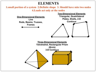
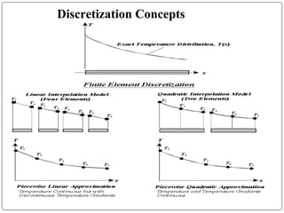
- Domain Discretization
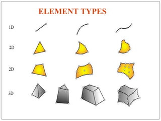
- Select Element Type (Shape and Approximation)
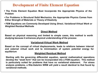
- Derive Element Equations (Variational and Energy Methods)
- Assemble Element Equations to Form Global System
[K]{U} = {F}
[K] = Stiffness or Property Matrix
{U} = Nodal Displacement Vector
{F} = Nodal Force Vector
- Incorporate Boundary and Initial Conditions
- Solve Assembled System of Equations for Unknown Nodal
Displacements and Secondary Unknowns of Stress and
Strain Values
19. TOPICS COVERED
⚫ GENERIC FORM OF FINITE
ELEMENT EQUATIONS
1.RAYLEIGH RITZ METHOD
2. WEIGHTED RESIDUAL
METHOD
3.BAR ELEMENT.
20.
21. One Dimensional Examples
Static Case
1 2
u1
u2
Bar Element
Uniaxial Deformation of Bars
Using Strength of Materials
Theory
Beam Element
Deflection of Elastic Beams
Using Euler-Bernouli Theory
1 2
w1
w2
θ2
θ1
22. GENERAL STEPS OF THE FINITE ELEMENT
ANALYSIS
⚫ Discretization of structure > Numbering of Nodes
and Elements > Selection of Displacement
function or interpolation function > Define the
material behavior by using Strain – Displacement
and Stress – Strain relationships > Derivation of
element stiffness matrix and equations >
Assemble the element equations to obtain the
global or total equations > Applying boundary
conditions > Solution for the unknown
displacements > computation of the element
strains and stresses from the nodal displacements
23. Advantages of Finite Element Method
⚫ 1. FEM can handle irregular geometry in a
convenient manner.
⚫ 2. Handles general load conditions without
difficulty
⚫ 3. Non – homogeneous materials can be handled
easily.
⚫ 4. Higher order elements may be implemented.
Disadvantages of Finite Element Method
⚫ 1. It requires a digital computer and fairly extensive
⚫ 2. It requires longer execution time compared with
24. APPLICATIONS OF FINITE ELEMENT ANALYSIS
⚫ Structural Problems:
⚫ 1. Stress analysis including truss and frame analysis
⚫ 2. Stress concentration problems typically associated
with holes, fillets or other changes in geometry in a
body.
⚫ 3. Buckling Analysis: Example: Connecting rod
subjected to axial compression.
⚫ 4. Vibration Analysis: Example: A beam subjected to
different types of loading.
⚫ Non - Structural Problems:
⚫ 1. Heat Transfer analysis: Example: Steady state thermal
analysis on composite cylinder.
⚫ 2. Fluid flow analysis: Example: Fluid flow through
25. BASED ON FEA
What is ANSYS?
•General purpose finite element modeling package for numerically solving a
wide variety of mechanical problems.
What is meant by finite element?
•A small units having definite shape of geometry and nodes
What is the basic of finite element method?
•Discretization
State the three phases of finite element method.
• Preprocessing ,Analysis ,Post Processing
State the methods of engineering analysis?
•Experimental ,Analytical methods
What are the h versions of finite element method?
•The order of polynomial approximation for all elements and numbers of
elements are kept increased
What is Discretization?
The art of dividing a structure in to a convenient number of smaller components
Defining the Job name
Utility Menu>File>Change Job name
26. BASED ON FEA AND ANSYS
What is the effect of size and number of elements on the solution by
FEM.?
•Smaller size and more no. elements more FEA accuracy
How to improve accuracy of solution by FEM?
•By increasing no. of elements , by fine meshing, by choosing higher order
polynomial function
What is DOF?
•It is a variable that describes the behavior of a node in an element.
What is meshing?
•The minimum number of elements that give you a converged solution.
In how many methods ANSYS can be used?
•Graphical User Interface or GUI and Command files
What kind of hardware do need to run a ANSYS?
•A PC with a sufficiently fast processor, at least 2GB RAM, and at least 500 GB
of hard disk
Name any FEA software
1.ANSYS 2.NASTRAN 3.COSMOS 4.NISA 5.ASKA 6.DYNA 6.I-DEAS
27. •Finite element analysis.
Finite element method is a numerical method for of engineering, mathematical,
physics. In the finite element method, instead of solving the problem for the entire
body in one operation, we formulate the equations for each finite element and
combine them to obtain the solution of the whole body
•Finite element
A small unit having definite shape of geometry and nodes is called finite element.
•State the methods of engineering analysis.
There are three methods of engineering analysis. 1) Experimental method.2) Analytical
method.3) Numerical method or Approximate method.
•Types of boundary conditions
There are two types of boundary conditions; they are Primary boundary condition
.Secondary boundary condition.
•Structural and Non-structural problem
Structural problem: In structural problems, displacement at each nodal point is
obtained. By using these displacement solutions, stress and strain in each element can
be calculated.
Non Structural problem: In non structural problem, temperatures or fluid pressure at
each nodal point is obtained. By using these values, Properties such as heat flow, fluid
flow, etc for each element can be calculated.
28. •Name the weighted residual methods.
1.Point collocation method.2. Sub domain collocation method.3.Least square method
4. Gale kin’s method
•Rayleigh Ritz method.
Rayleigh Ritz method is a integral approach method which is useful for solving complex
structural problems, encountered in finite element analysis
•Total potential energy.
The total potential energy π of an elastic body, is defined as the sum of total strain energy
U and potential energy of the external forces,(W).
Total potential energy, π = Strain energy (U) - Potential energy of the external forces (W).
•Compare essential boundary conditions and natural boundary conditions.
There are two types of boundary conditions. They are:
1.Primary boundary condition (or) Essential boundary condition the boundary condition,
which in terms of field variable, is known as primary boundary condition.
2.Secondary boundary condition or natural boundary conditions: The boundary
conditions, which are in the differential form of field variables, are known as secondary
boundary condition.
•Compare boundary value problem and initial value problem
The solution of differential equation is obtained for physical problems, which satisfies some
specified conditions known as boundary conditions. The differential equation together with
these boundary conditions, subjected to a boundary value problem. The differential
equation together with initial conditions subjected to an initial value problem.
29. •Give examples for essential (forced or geometric) and
non-essential (natural) boundary conditions.
•geometric boundary conditions are displacement, slopes, etc.
•natural boundary conditions are bending moment, shear force, etc.
•Node or Joint
Each kind of finite element has a specific structural shape and is
interconnected with the adjacent elements by nodal points or nodes. At the
nodes, degrees of freedom are located. The forces will act only at nodes
and not at any other place in the element
What is meant by DOF?
When the force or reaction acts at nodal point, node is deformation. The
deformation includes displacement, rotations, and/or strains. These are
collectively known as degrees of freedom (DOF).
What is aspect ratio?
Aspect ratio is defined as the ratio of the largest dimension of to the
smallest dimension. In many cases, as the aspect ratio increases, the
inaccuracy of the solution increases. The conclusion of many researches is
that the aspect ratio should be close to unity as possible.
30. What are h and p versions of finite element method?
h version and p versions are used to improve the accuracy of the finite element
method.
In h versions, the order of polynomial approximation for all elements is kept constant
and the number of elements is increased.
In p version, the number of elements is maintained constant and the order of
polynomial approximation of element is increased. During Discretization,
Mention the places where it is necessary to place a node.
The following places are necessary to place a node during discretization process.
1. Concentrated load-acting point.
2. Cross section changing point
3. Different material inters junction point
4. Sudden change in load point.
•Steps in FEM.
• Discretization
• Selection of the displacement models
• Deriving element stiffness matrices
• Assembly of overall equations/ matrices
• Solution for unknown displacements
• Computations for the strains/stresses