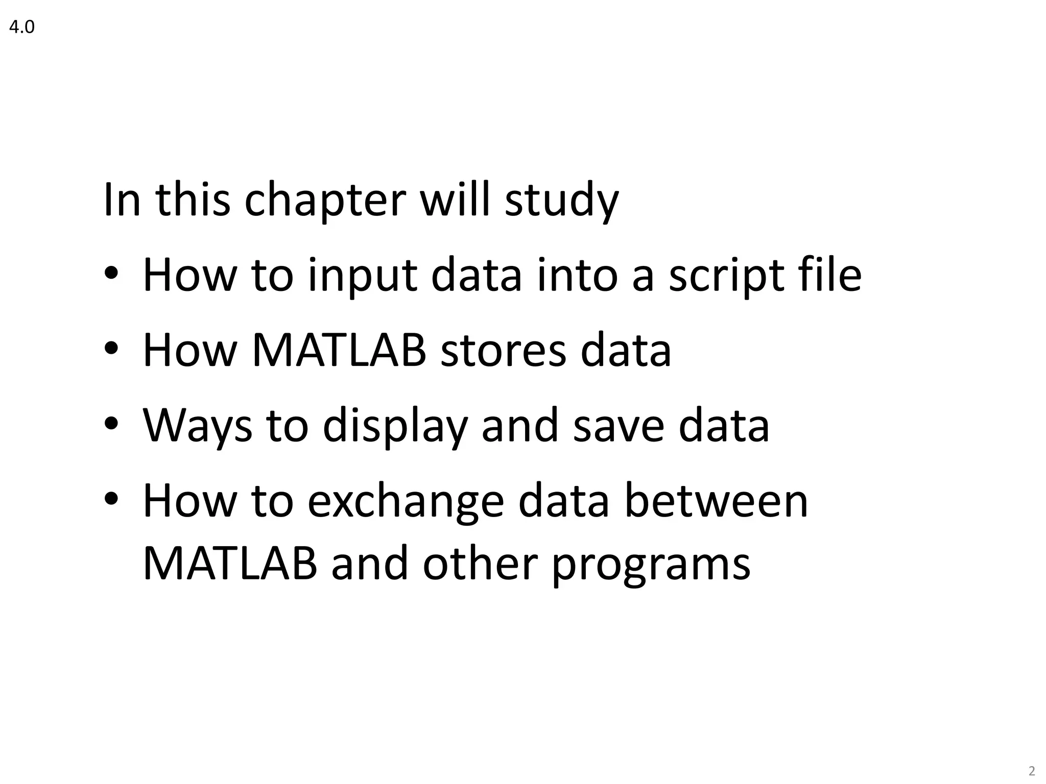
The chapter discusses inputting and managing data in MATLAB. It covers the MATLAB workspace, using script files to input data, displaying and saving output, and exchanging data with other programs. The key points are:
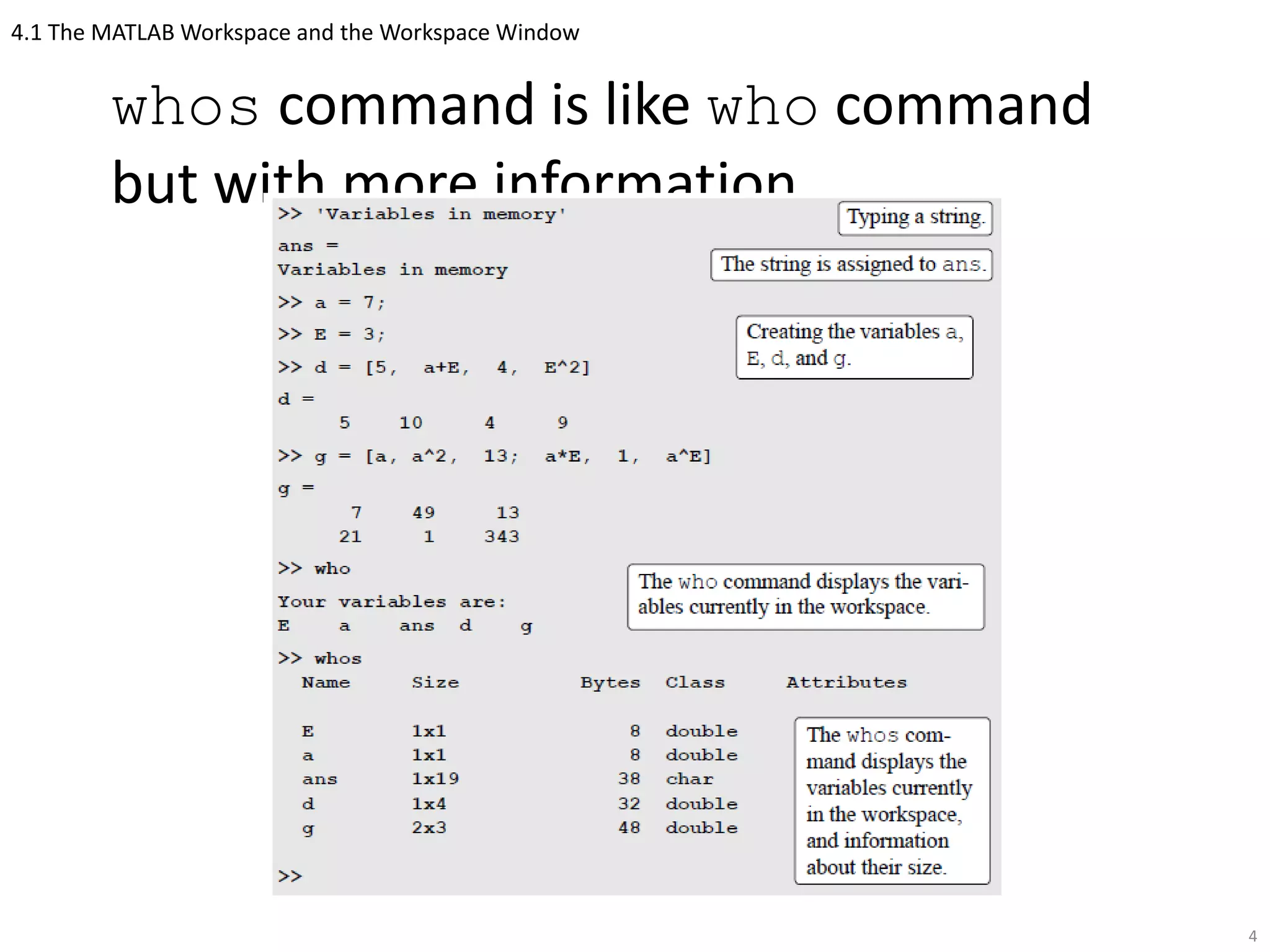
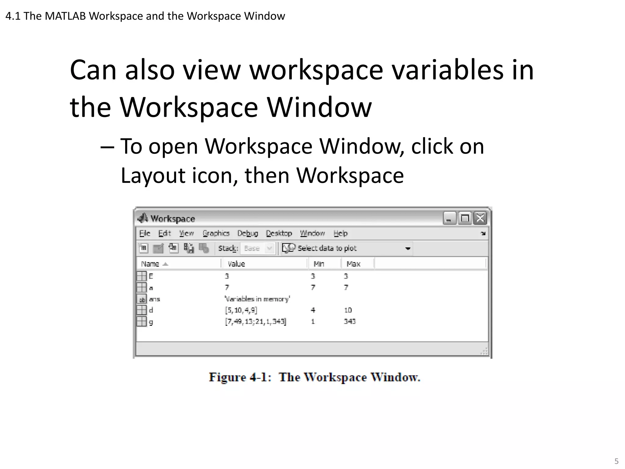
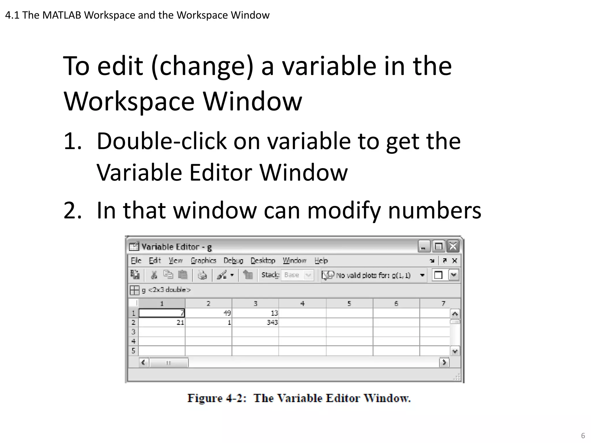
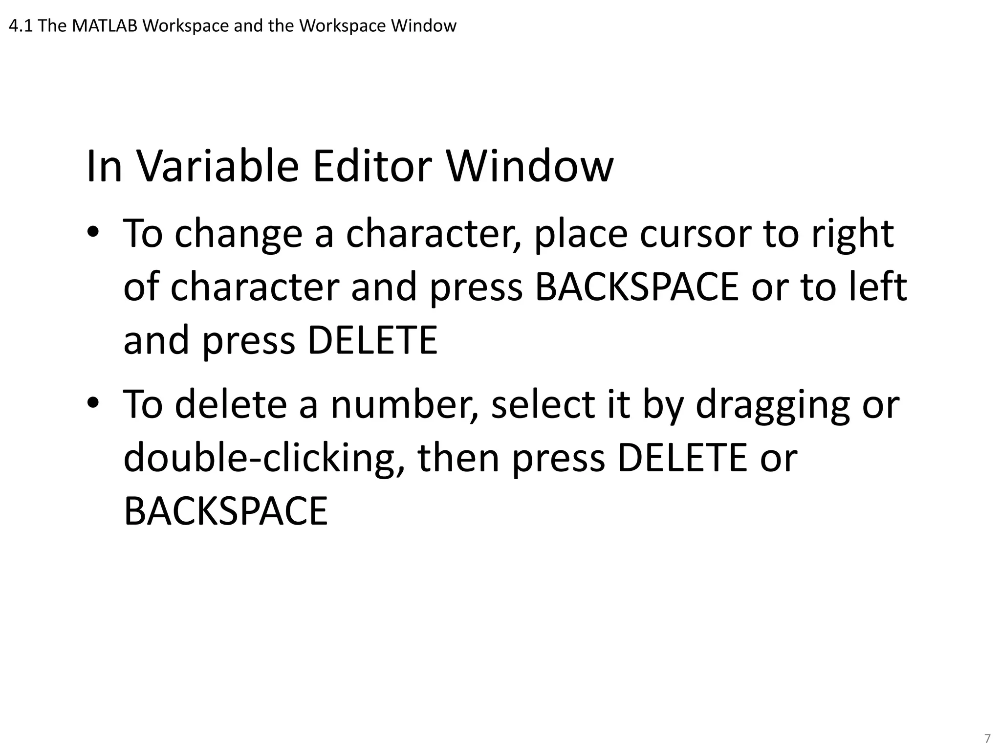
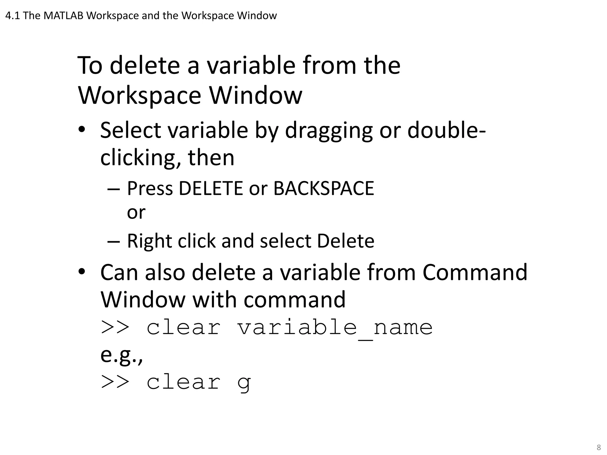
1) MATLAB stores variables in the workspace during a session and script files can access these variables. The workspace window allows viewing and editing variables.
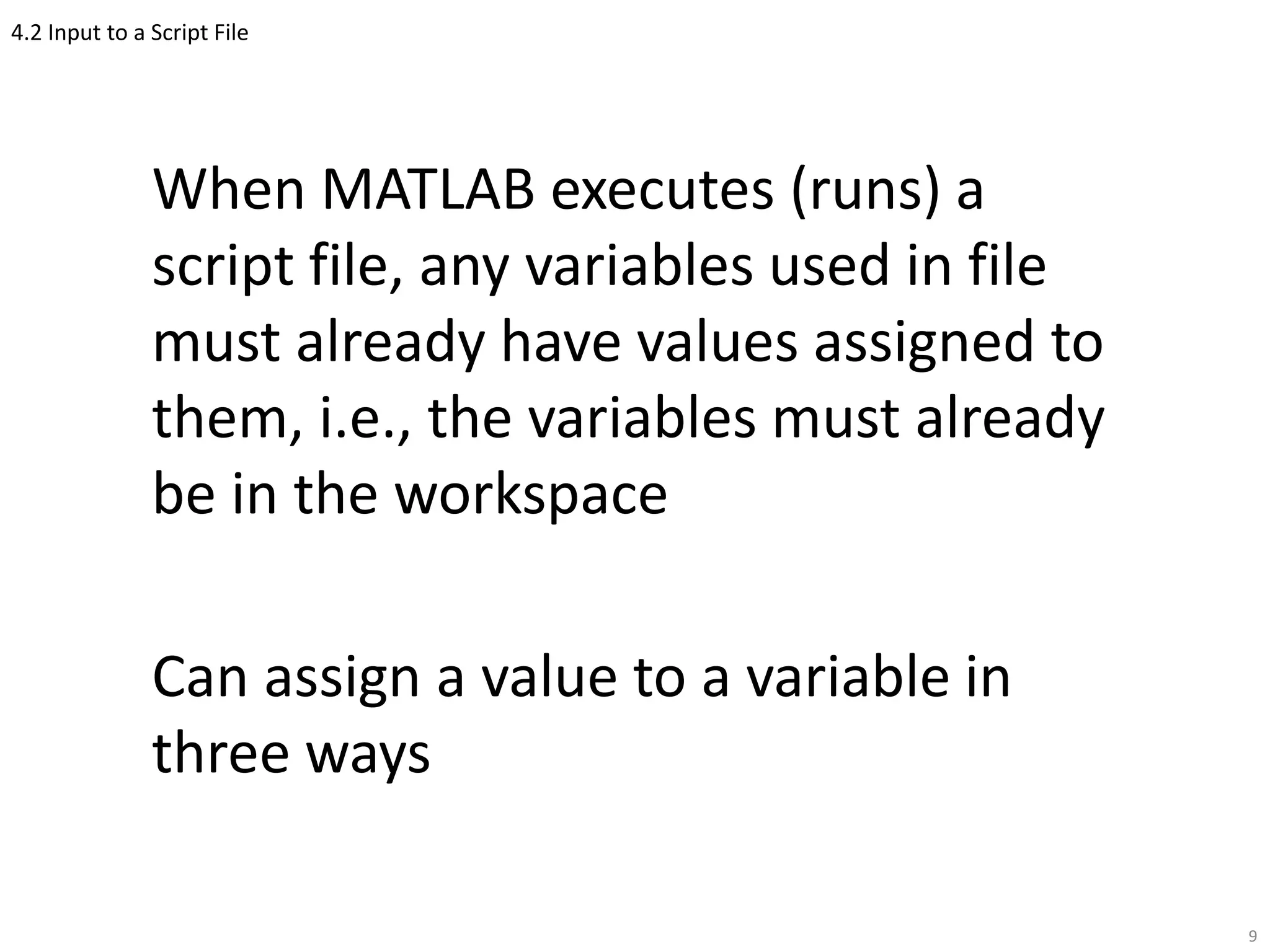
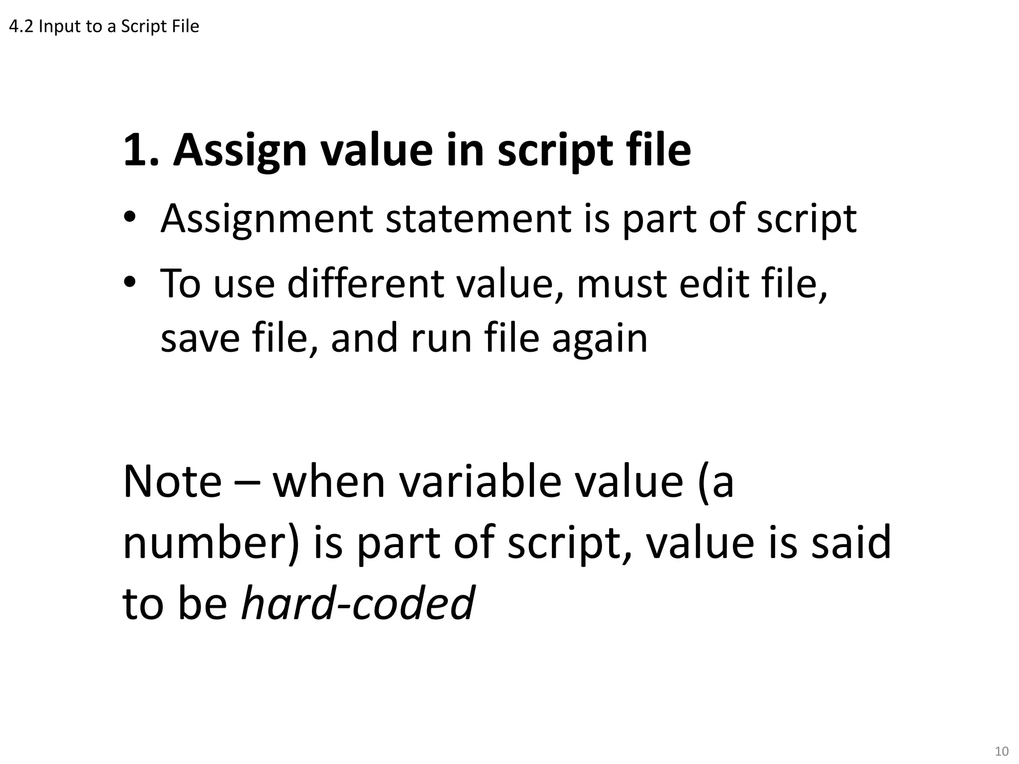
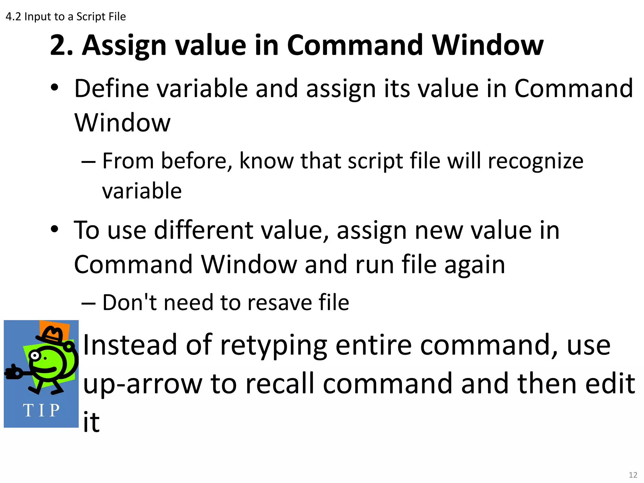
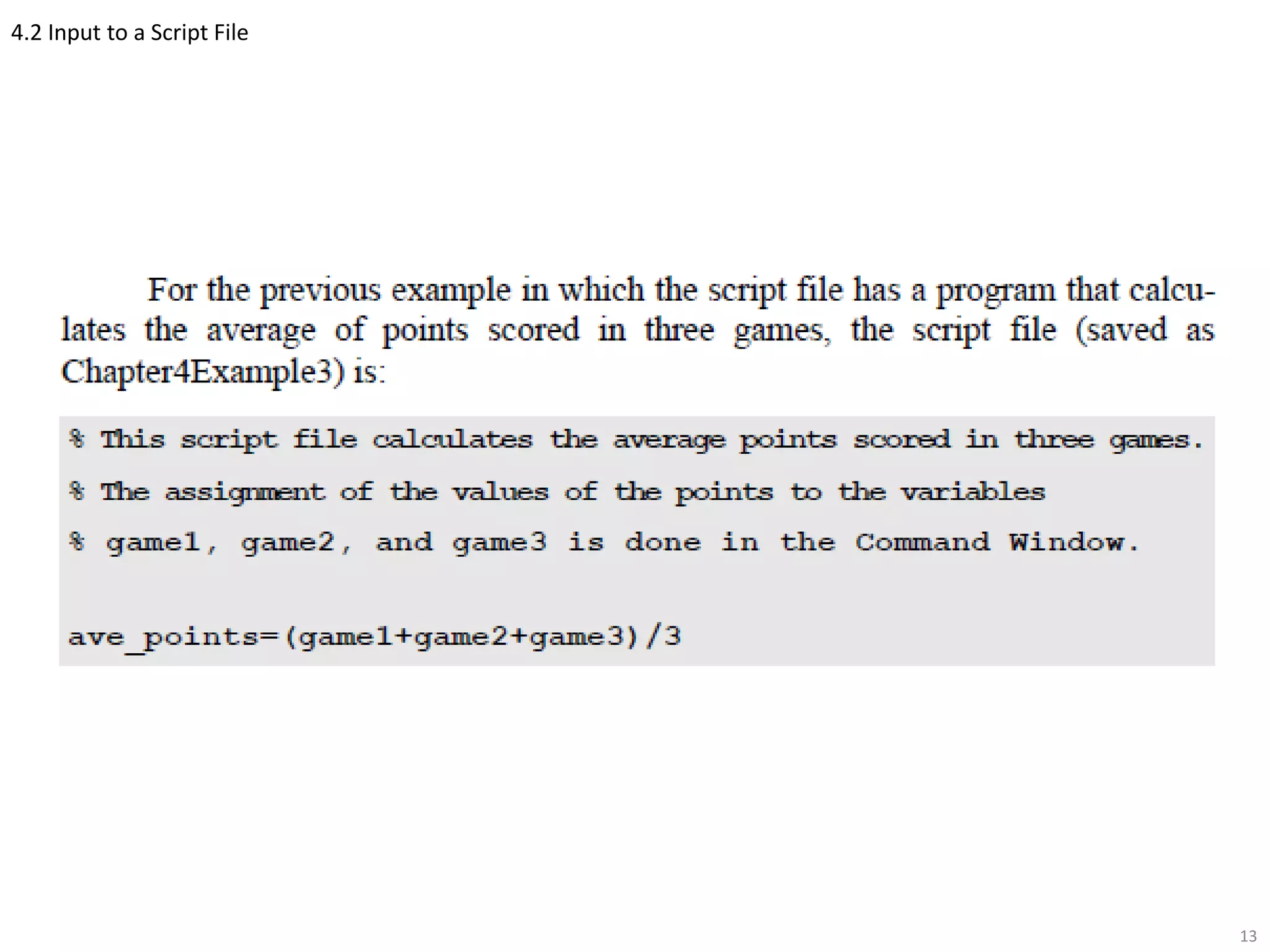
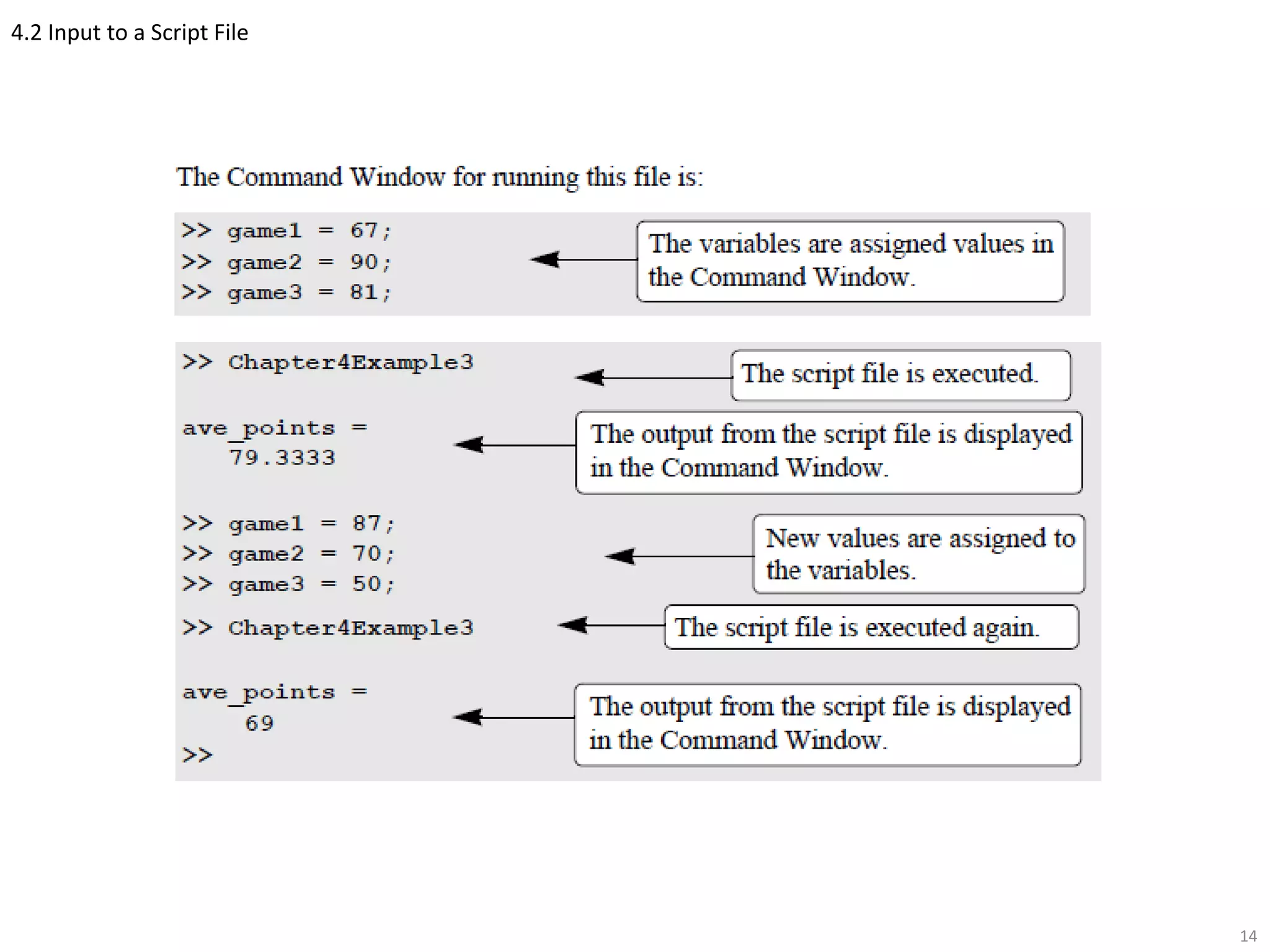
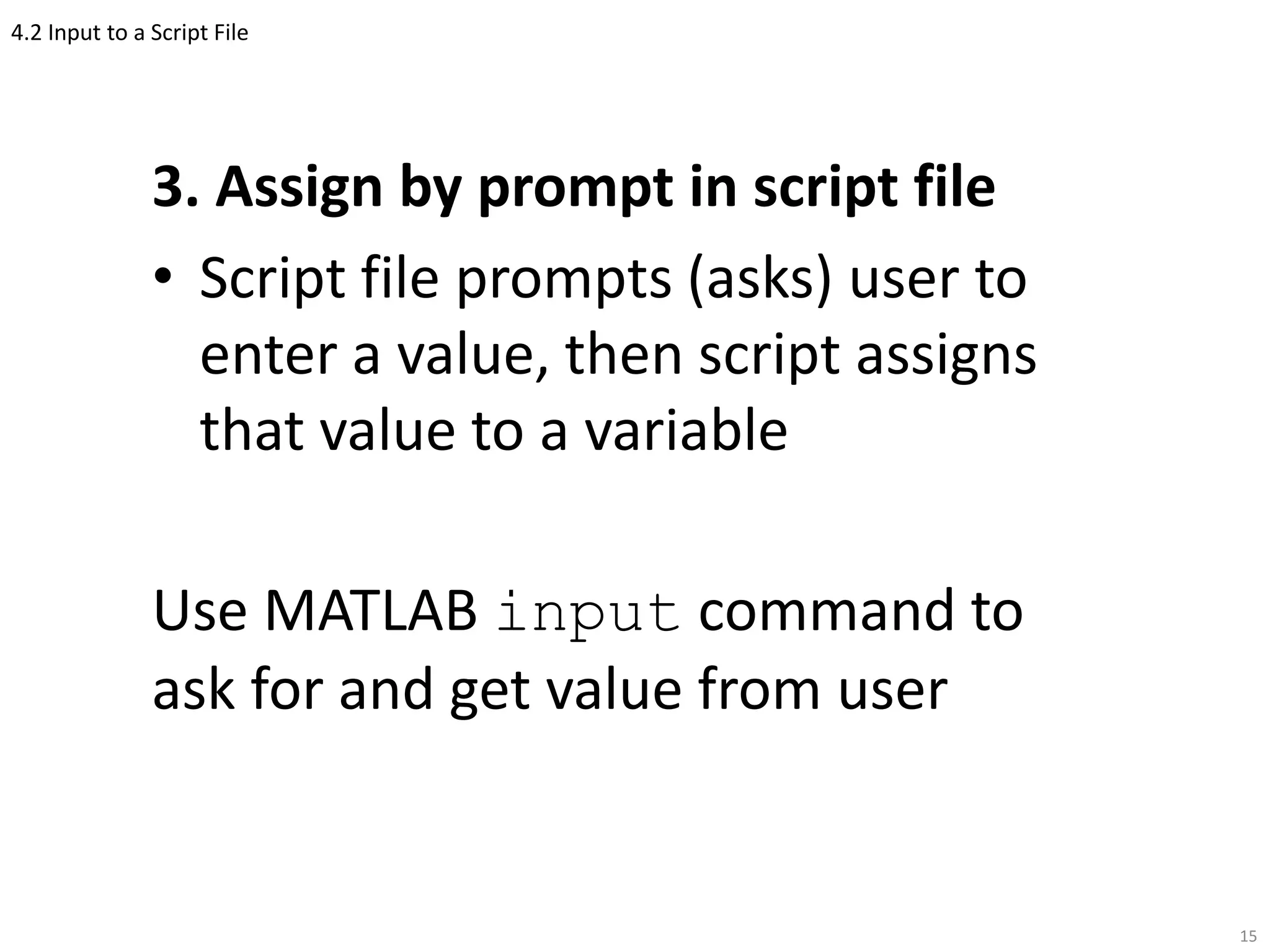
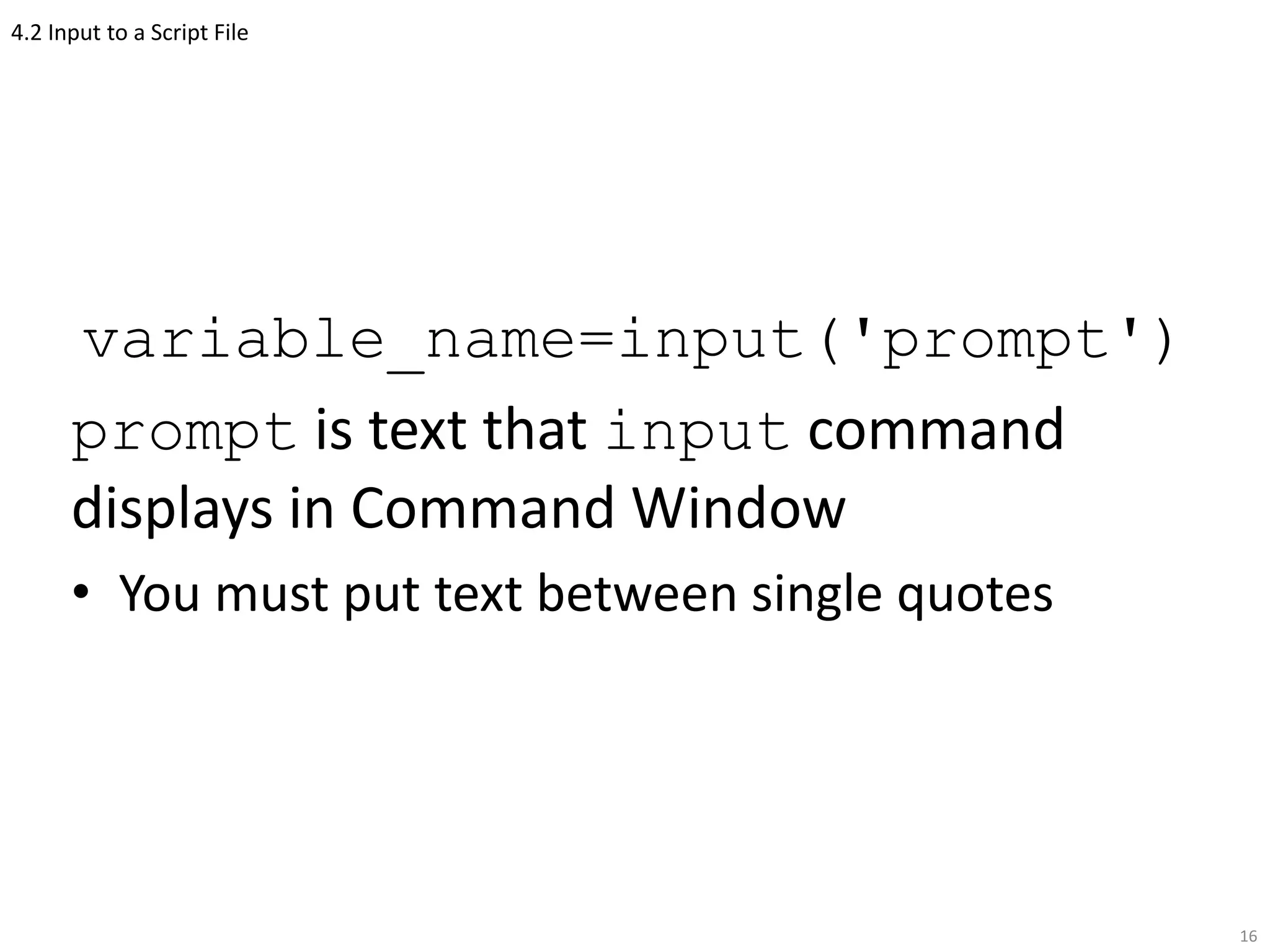
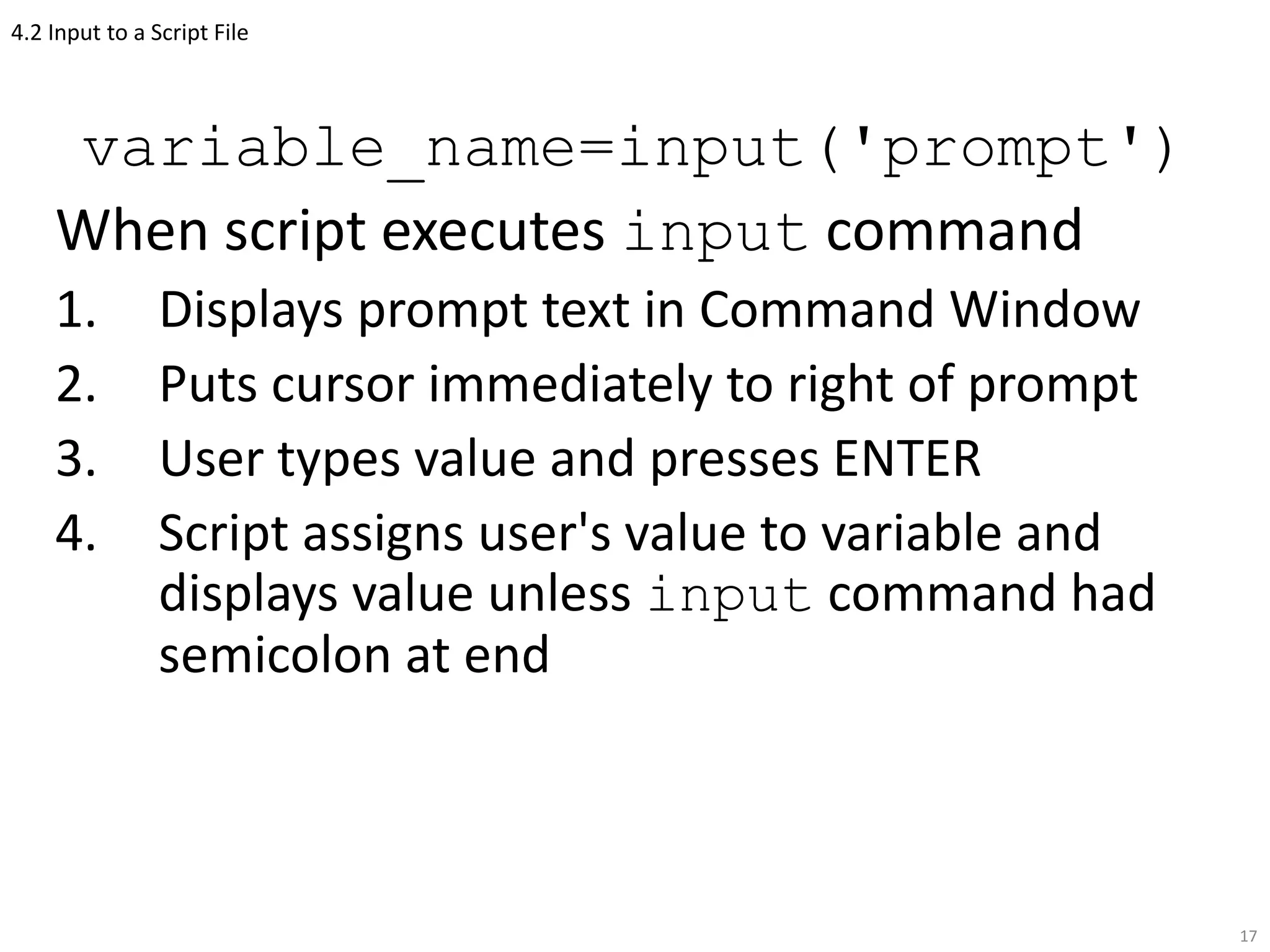
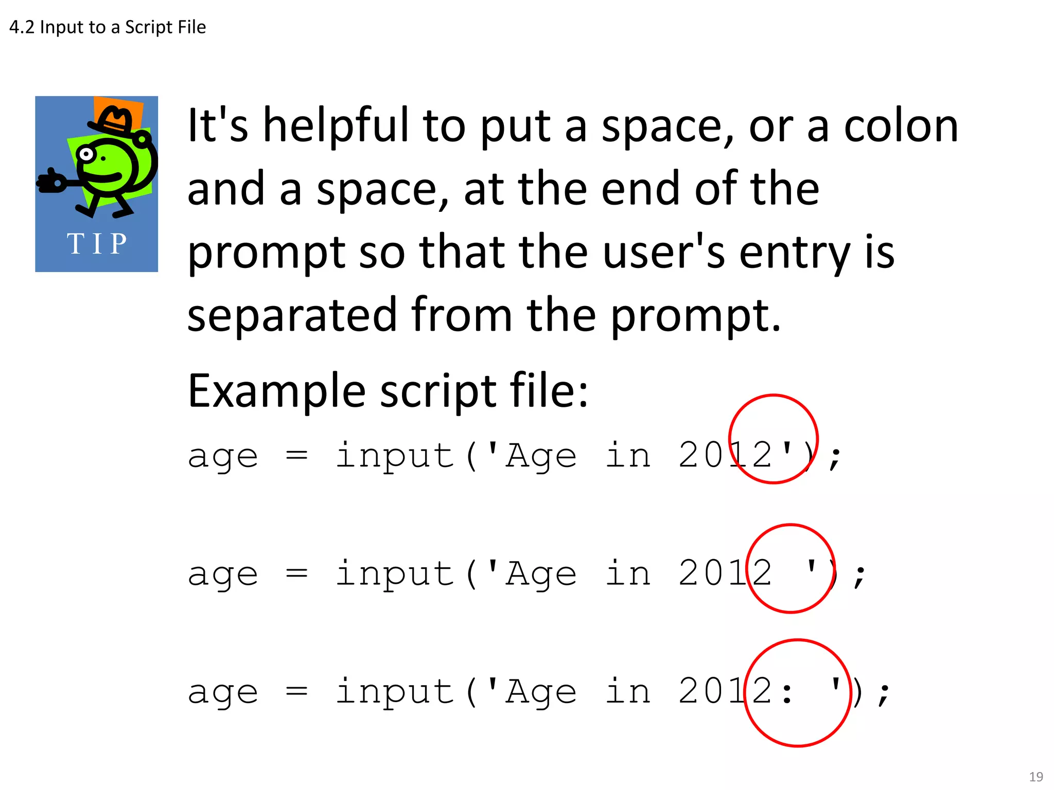
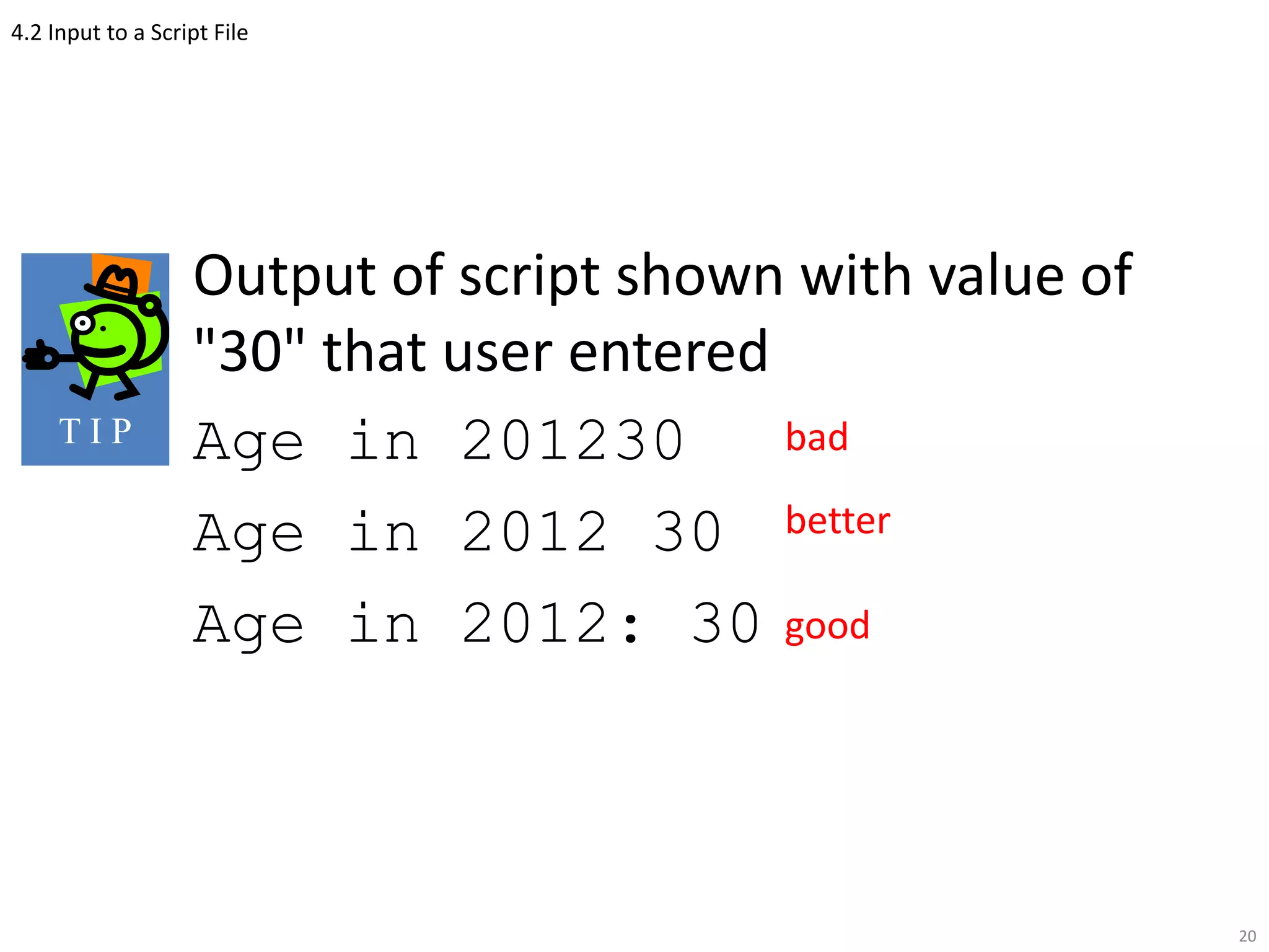
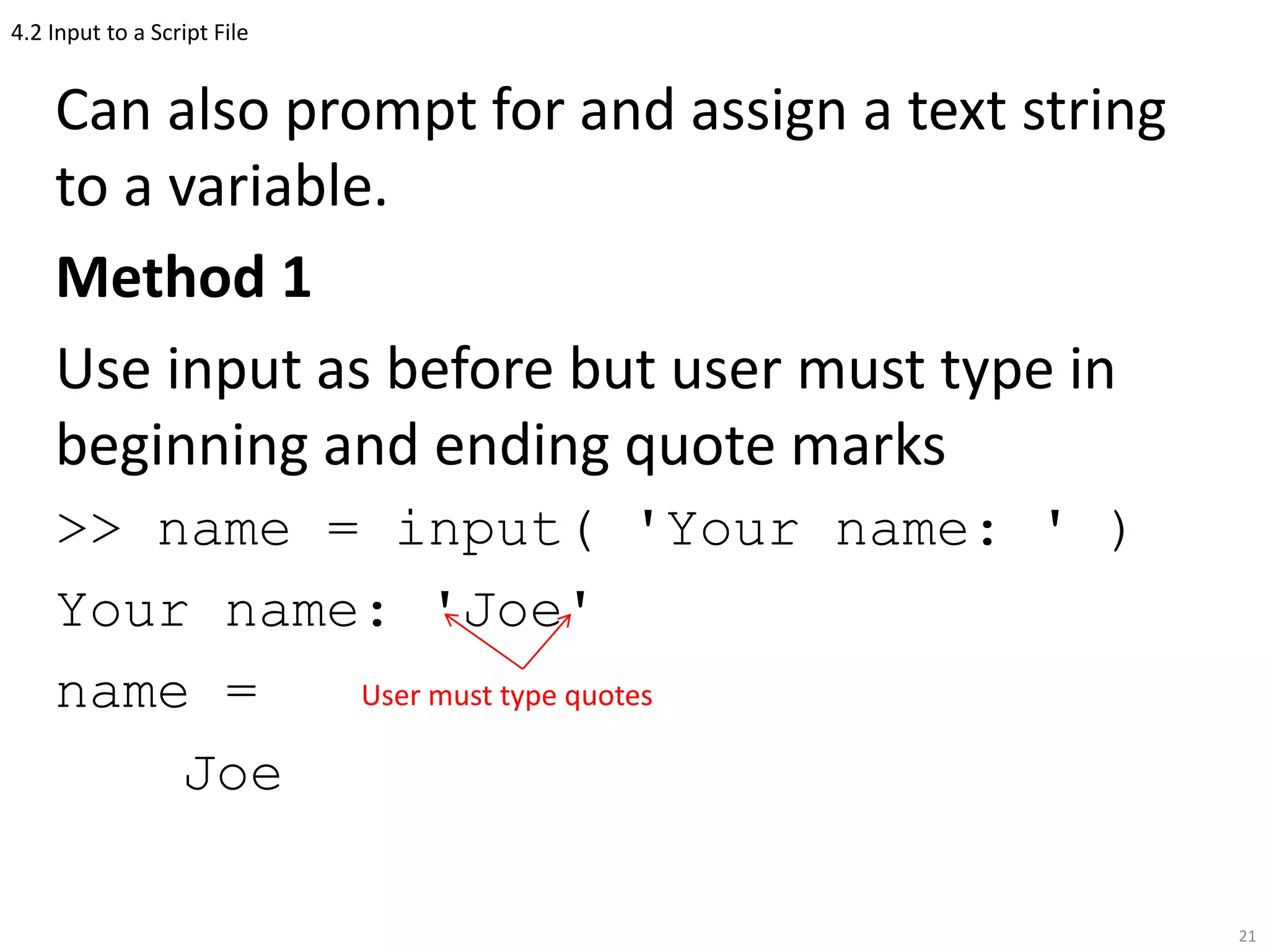
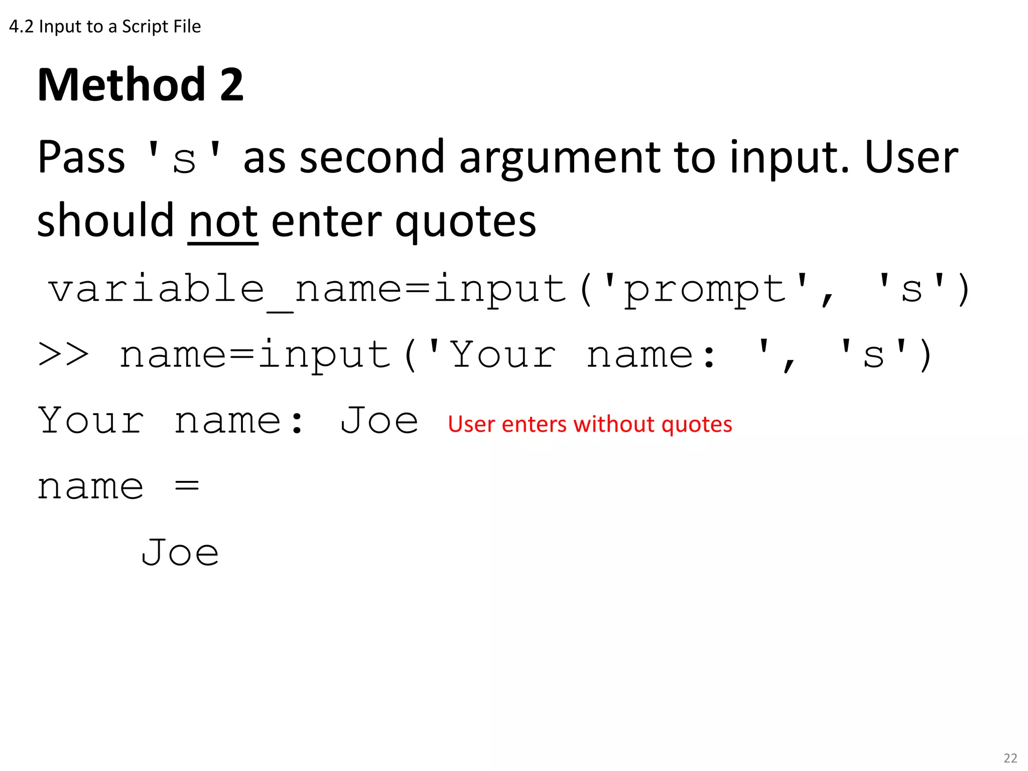
2) Script files can input data by assigning values in the file, command window, or prompting the user.
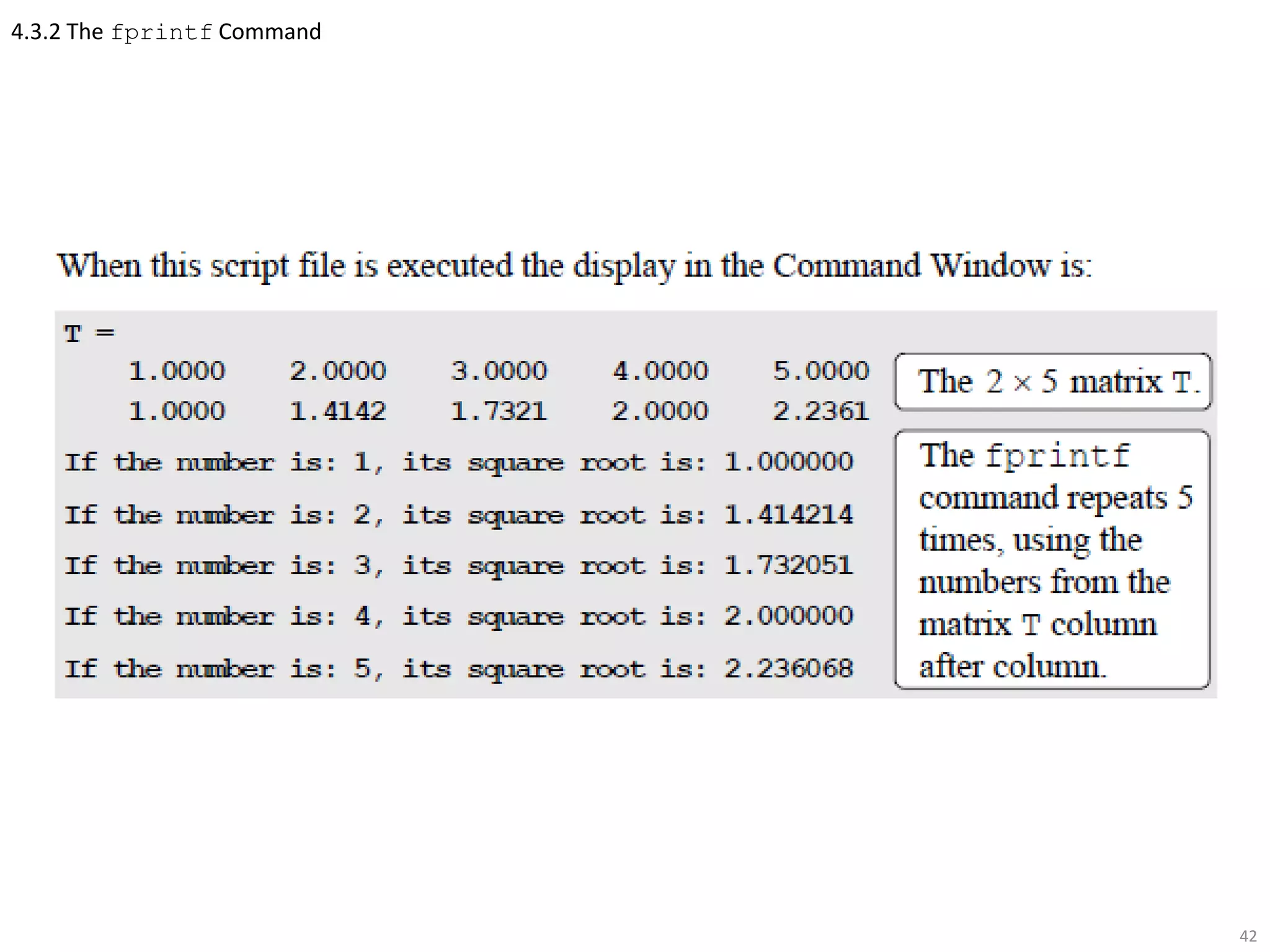
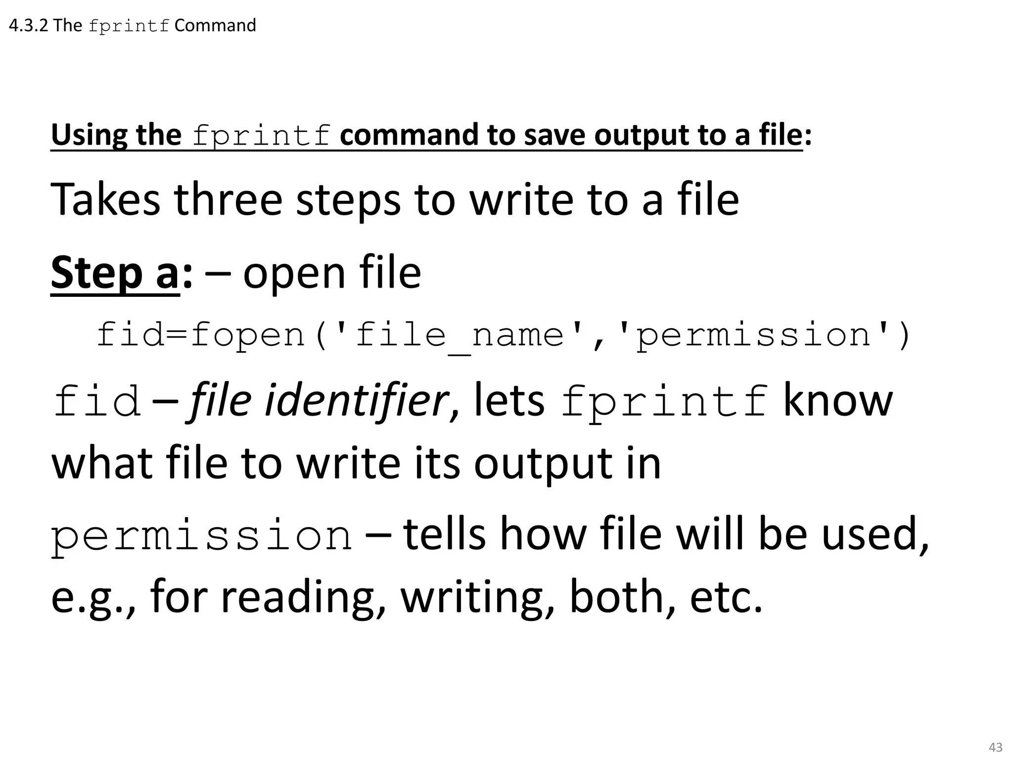
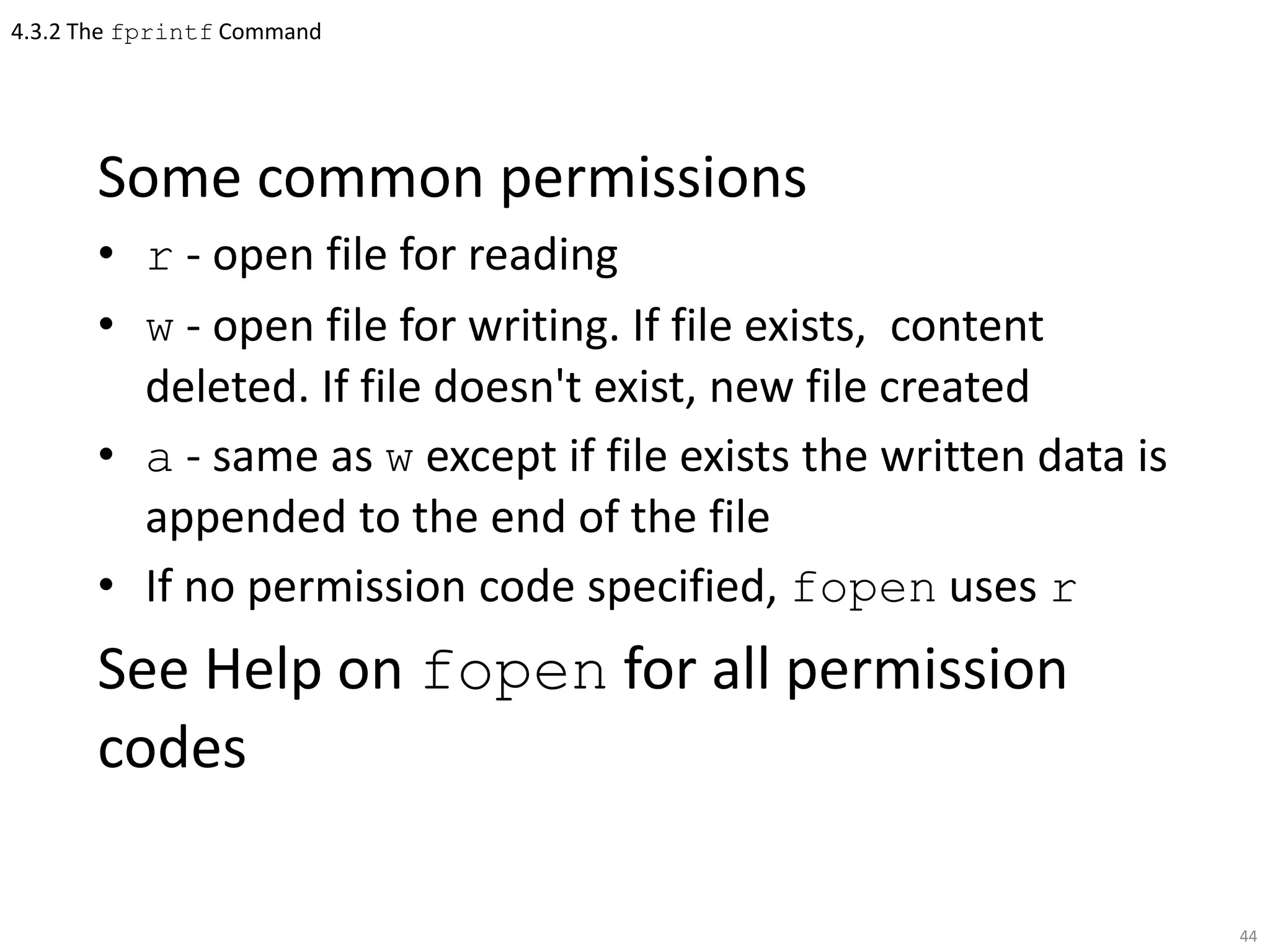
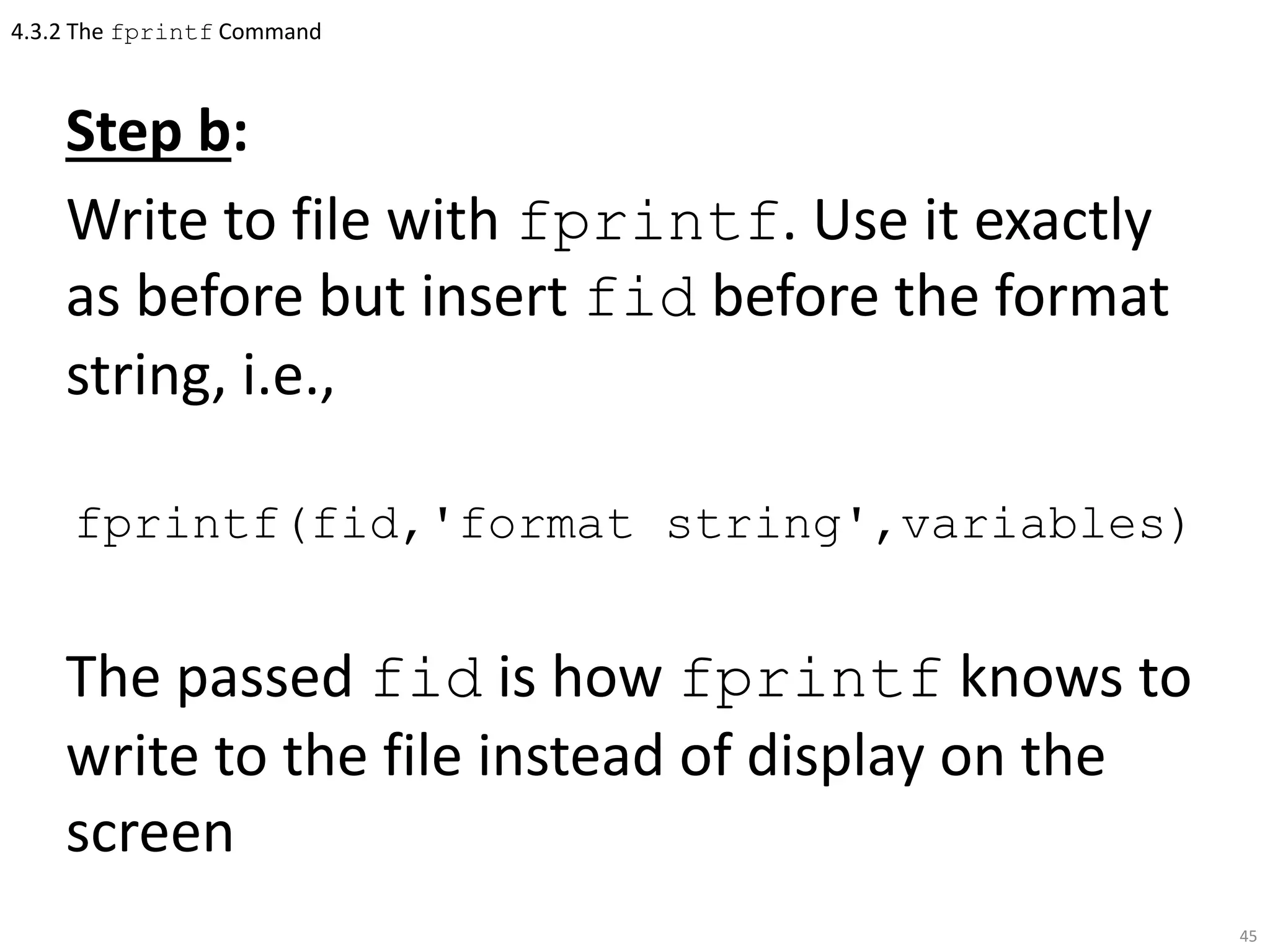
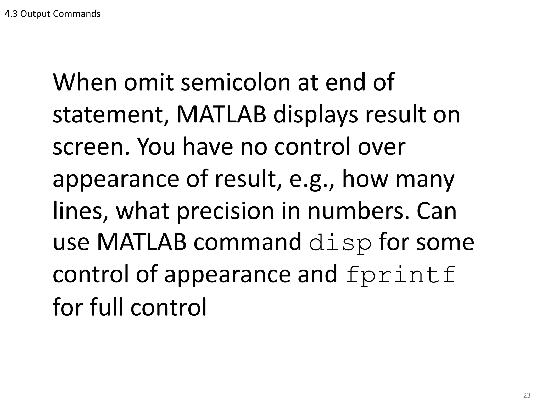
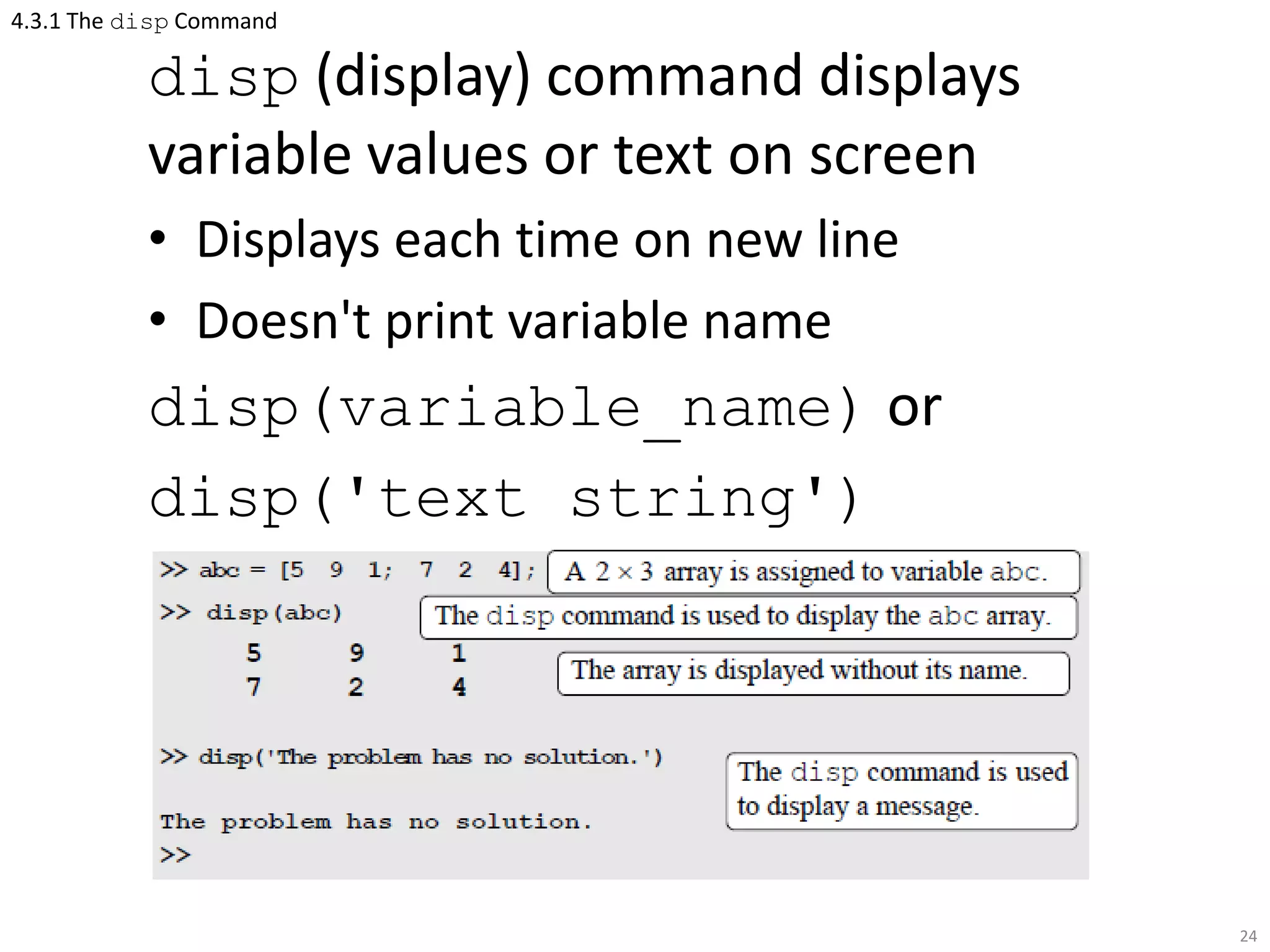
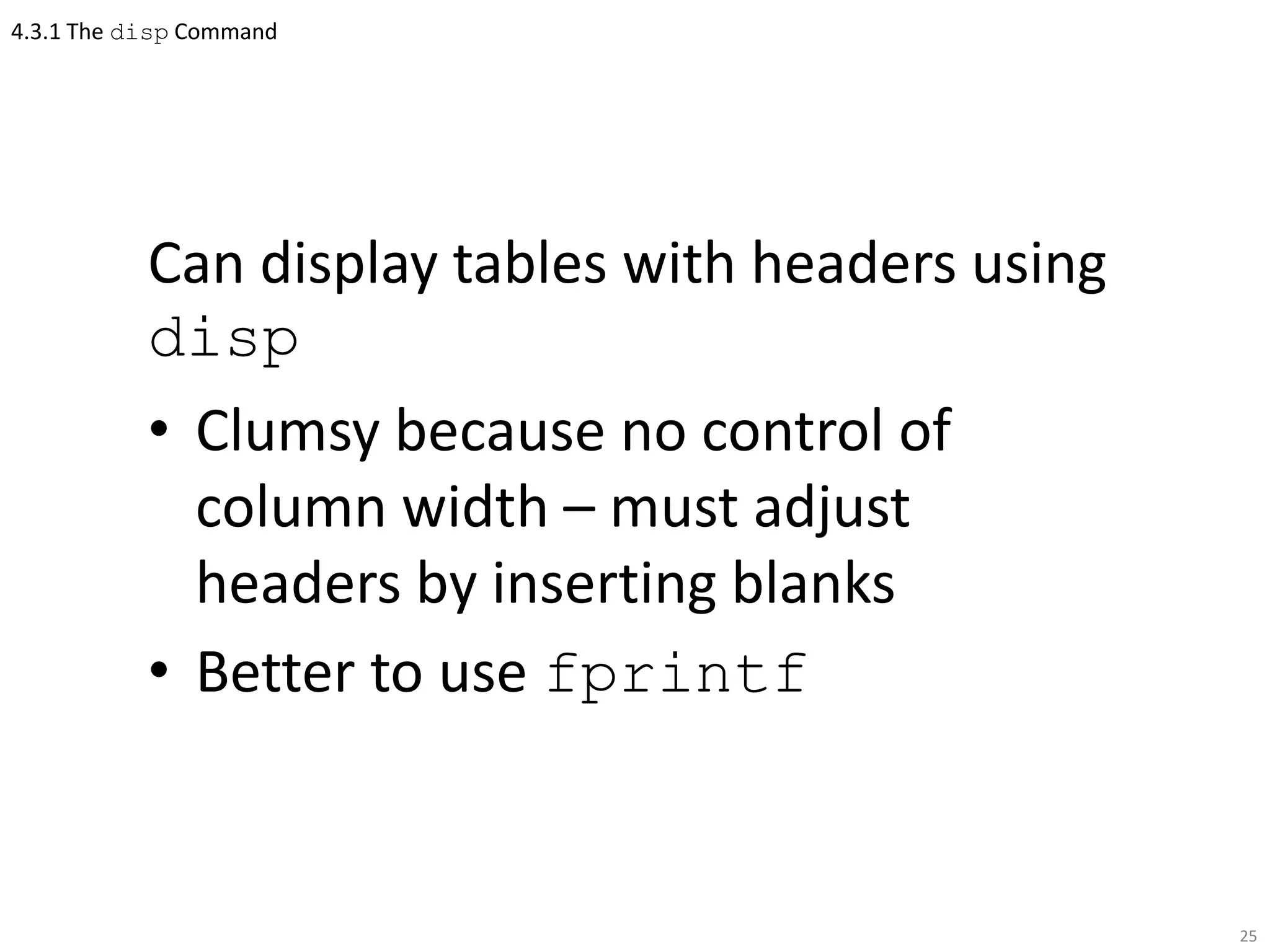
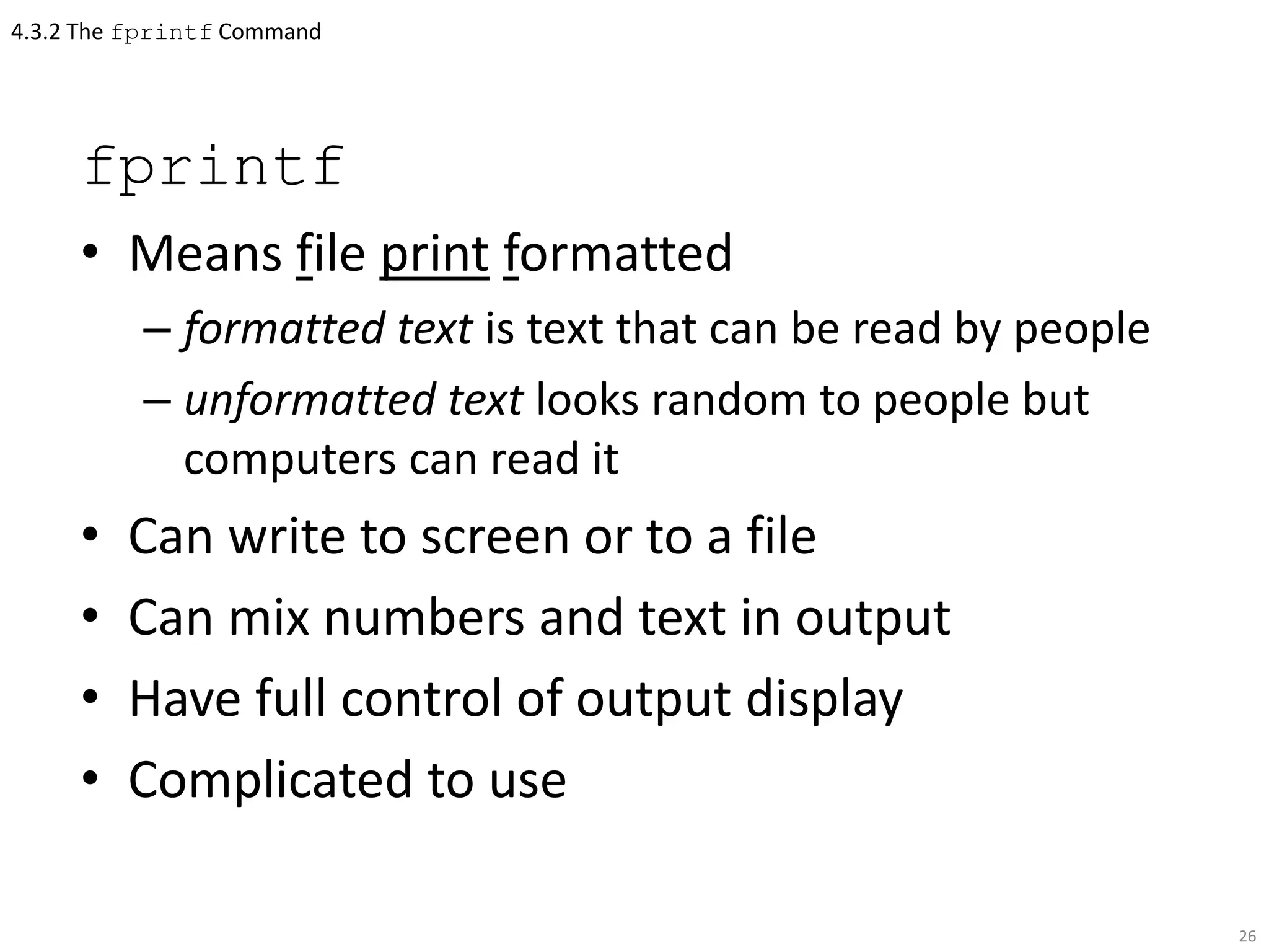
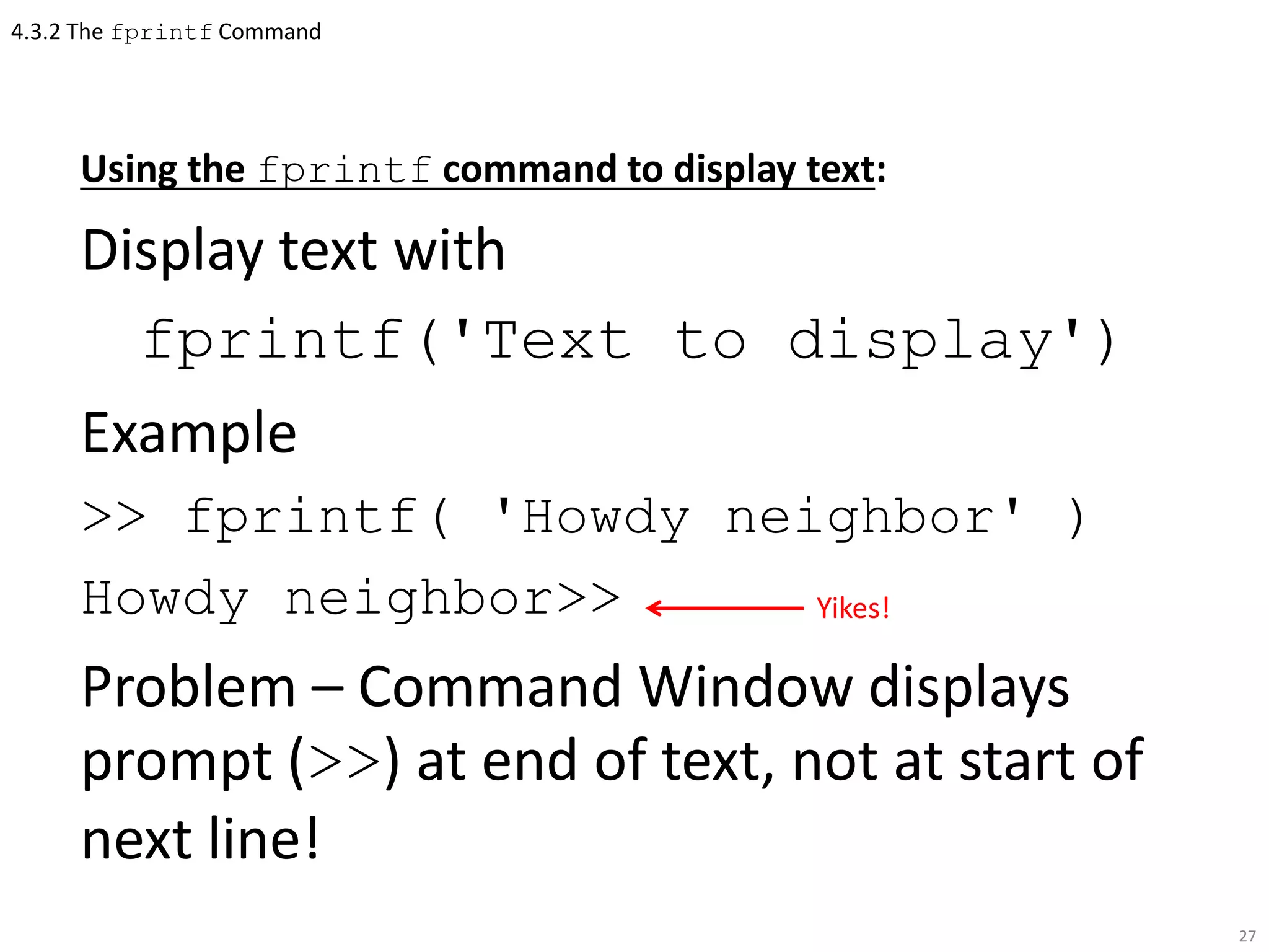
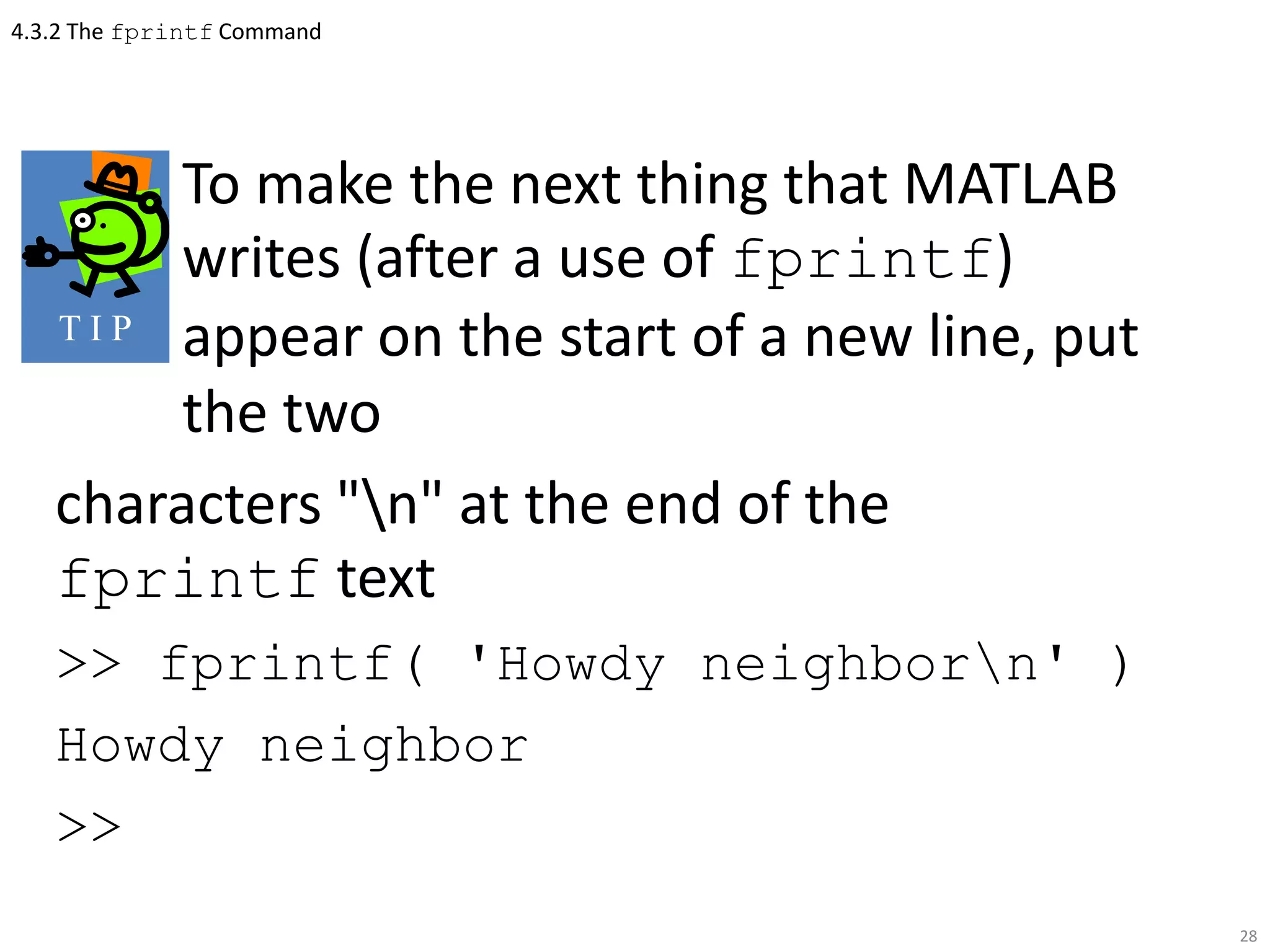
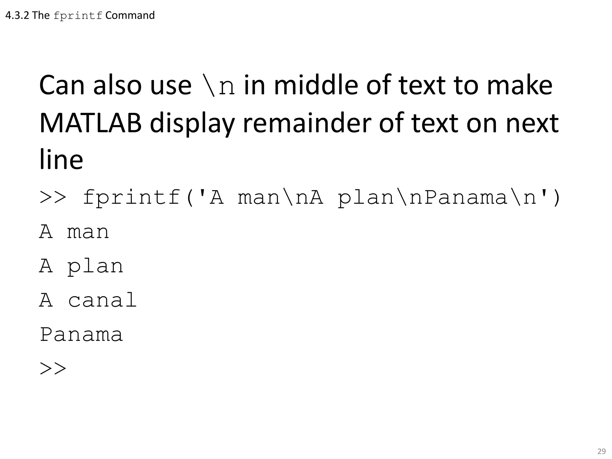
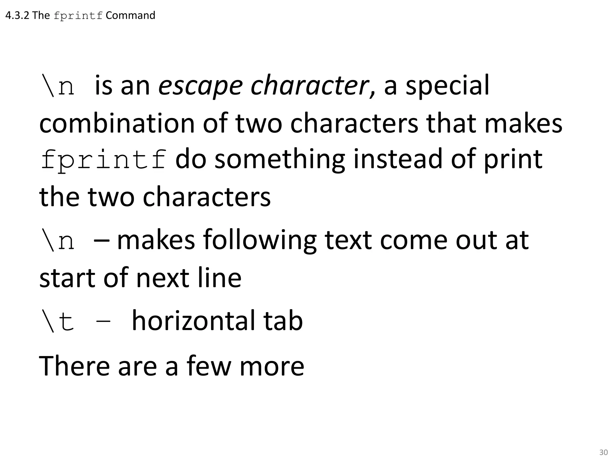
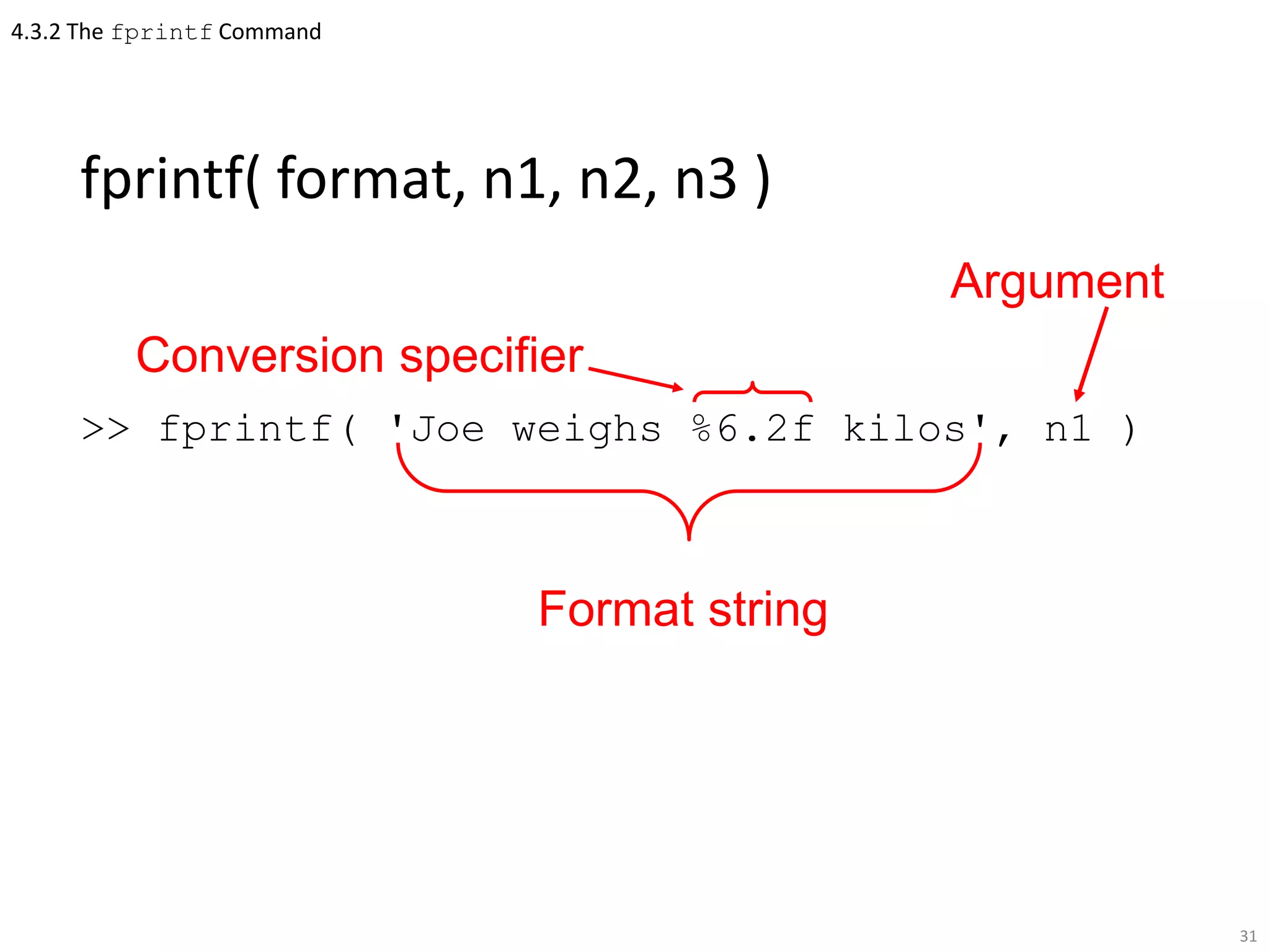
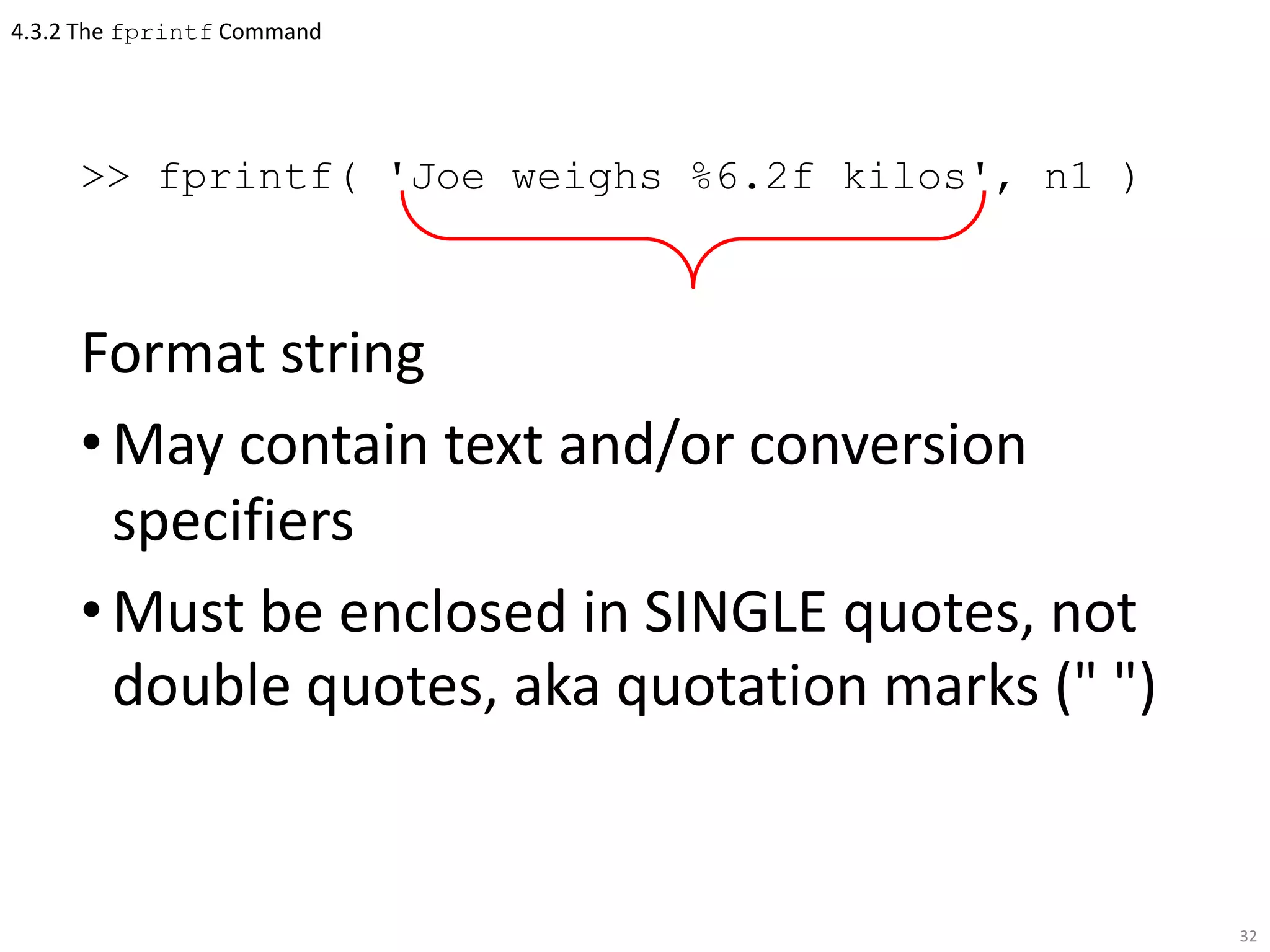
3) The disp and fprintf commands display output, with fprintf offering more formatting control. Fprintf can write to files or the screen.
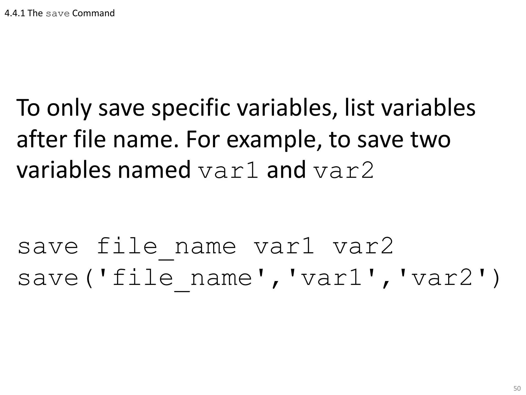
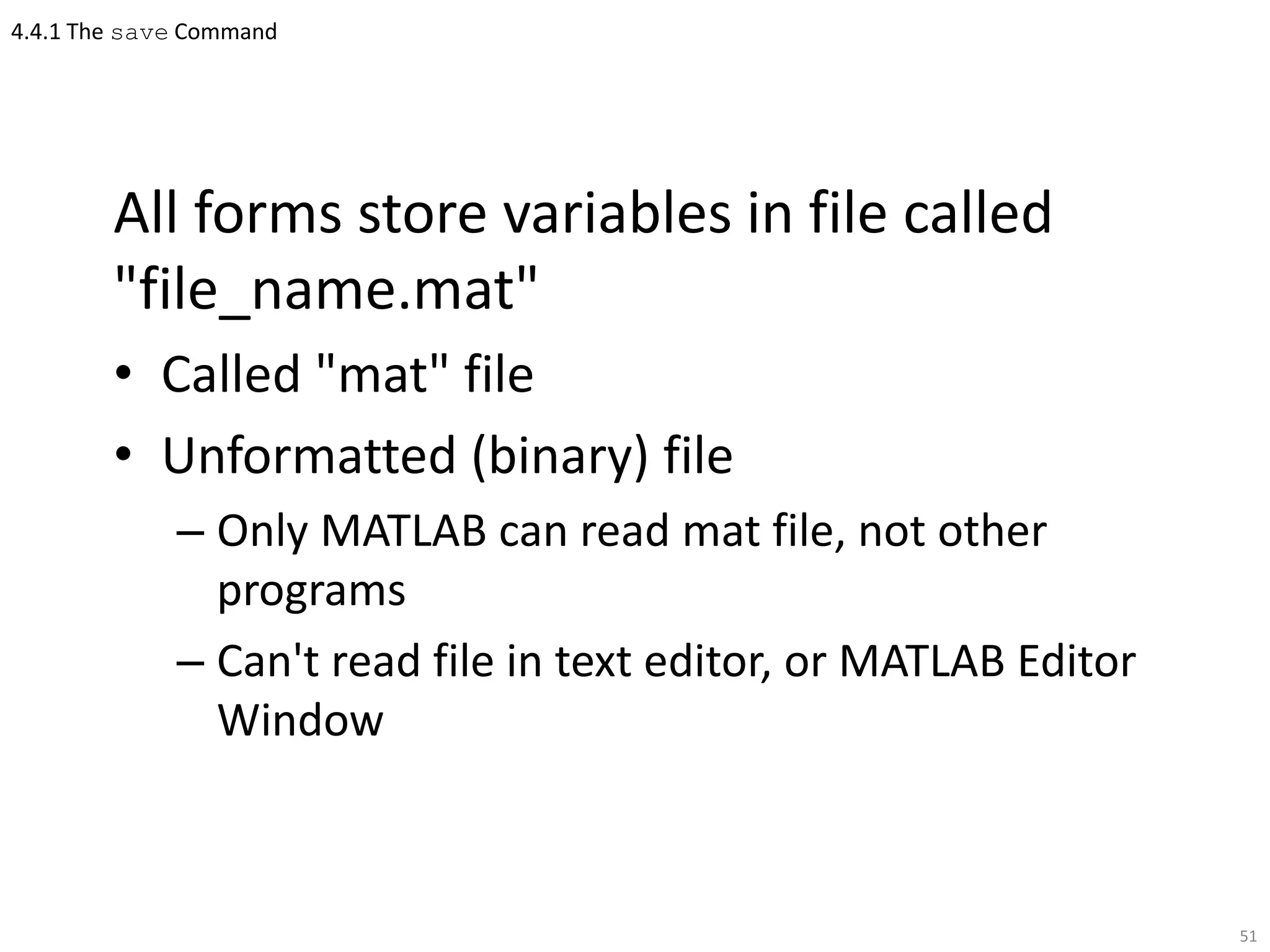
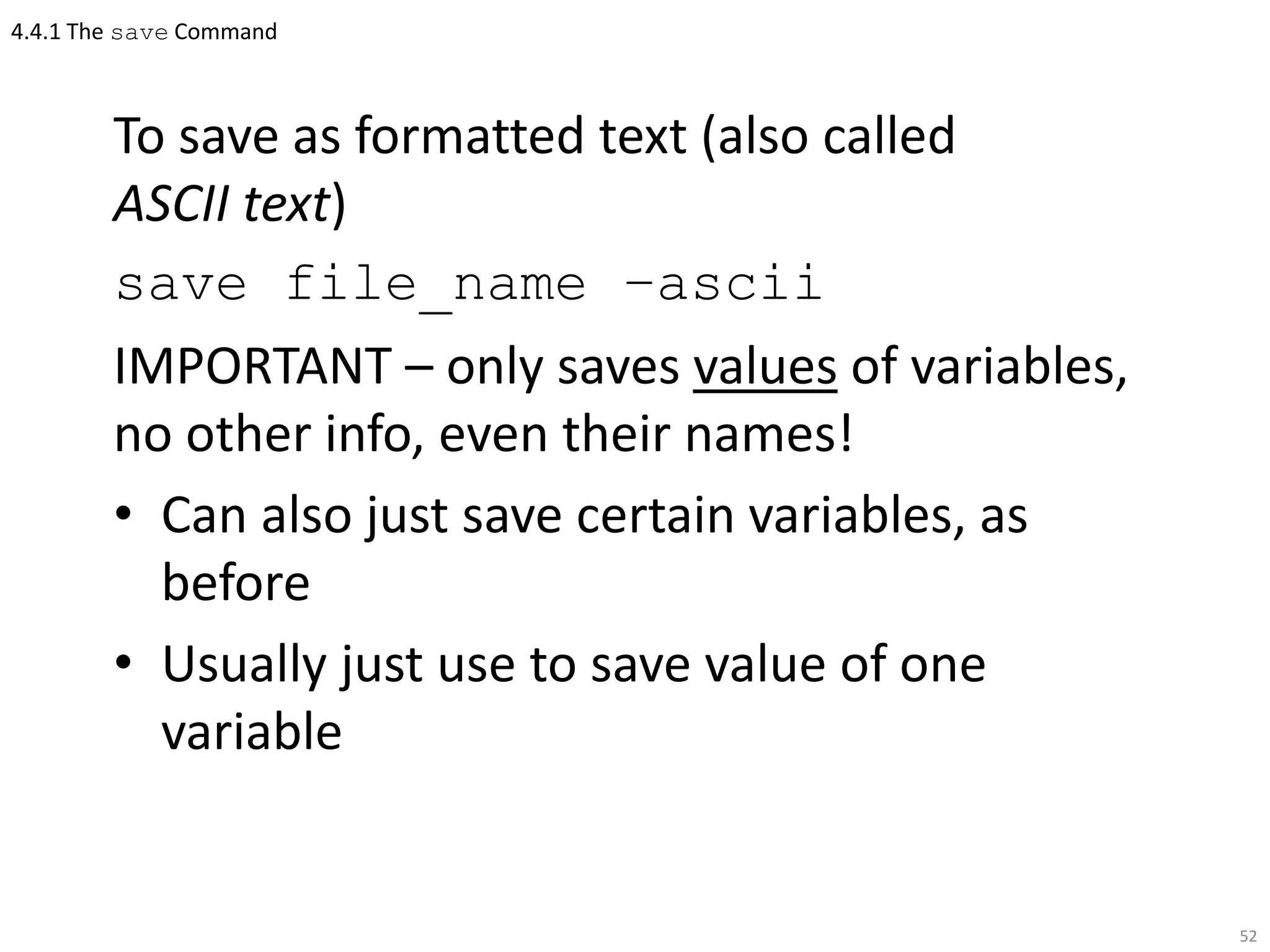
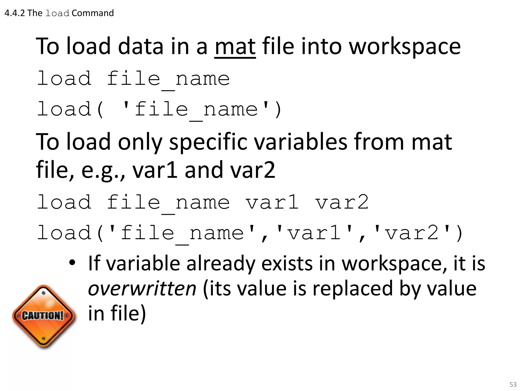
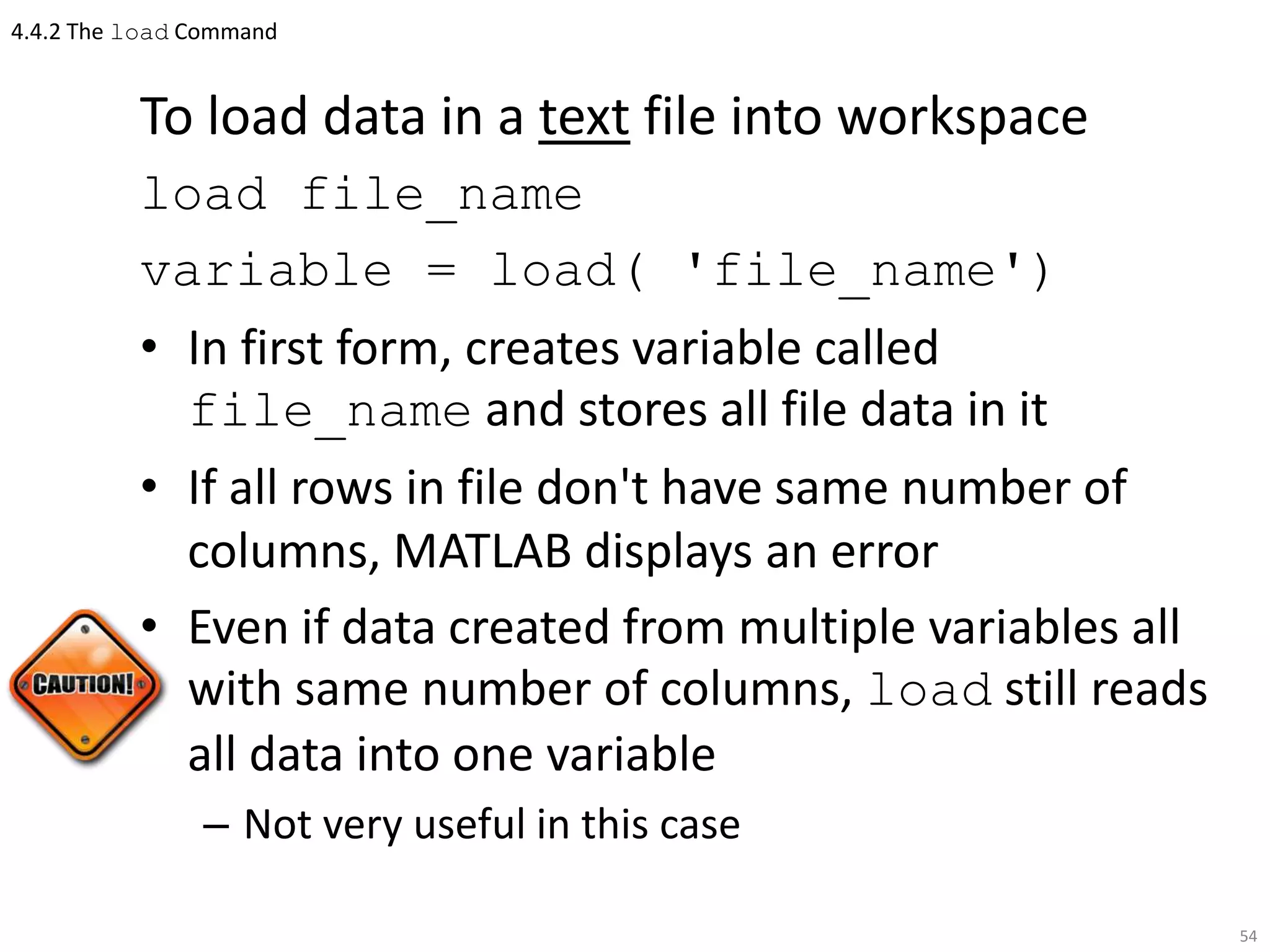
4) The save command saves workspace variables to a file, while load retrieves stored data
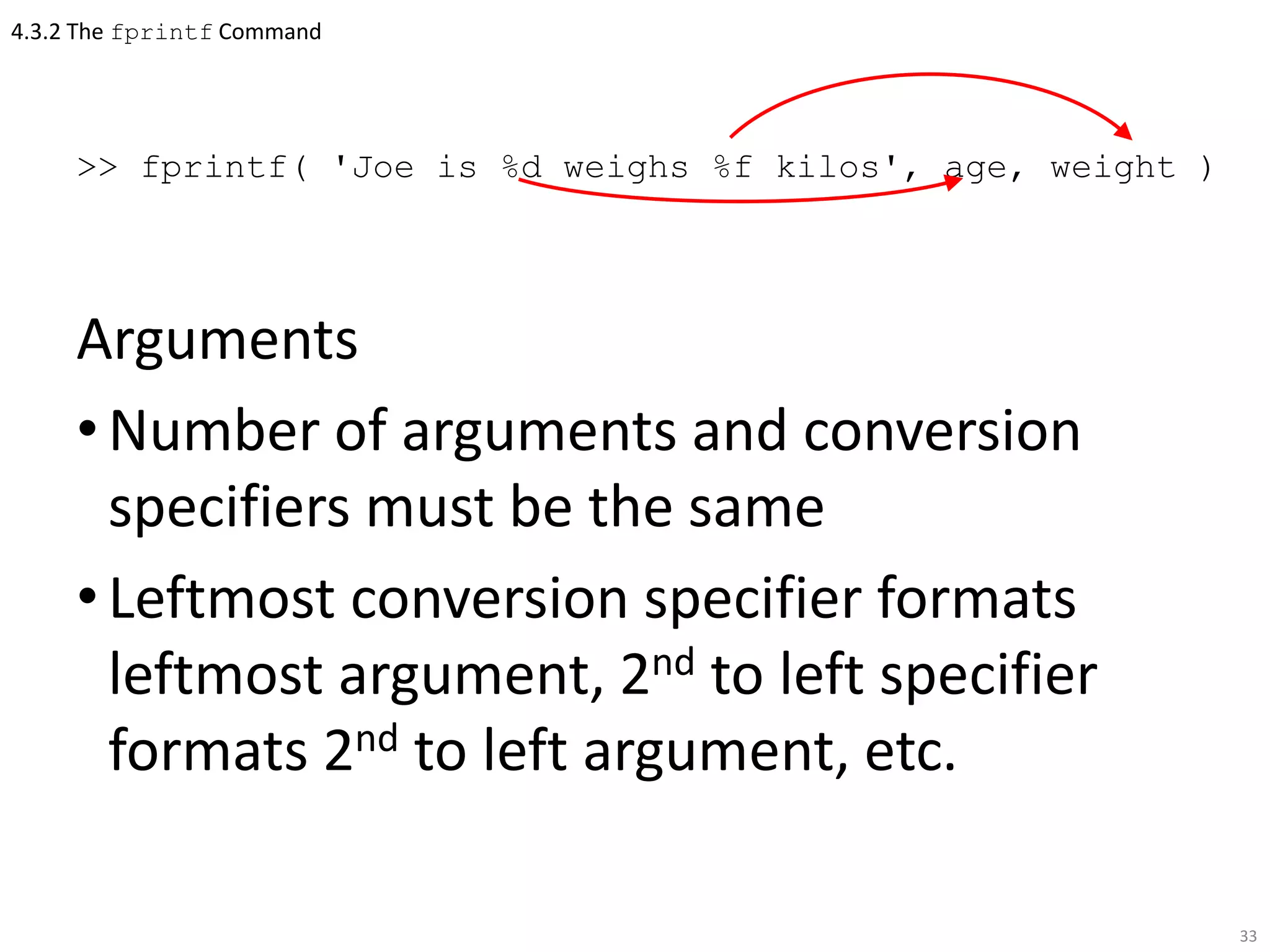
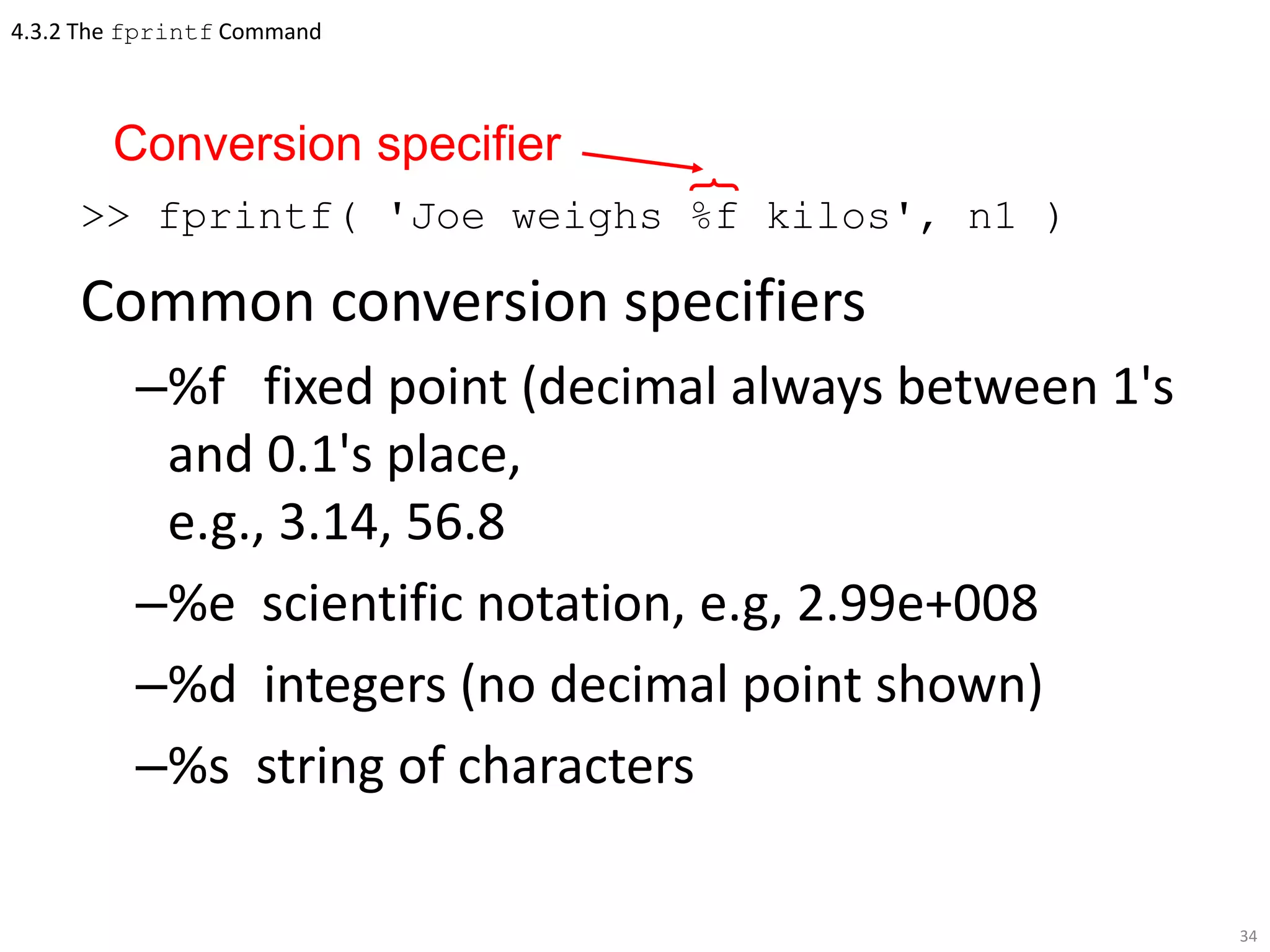
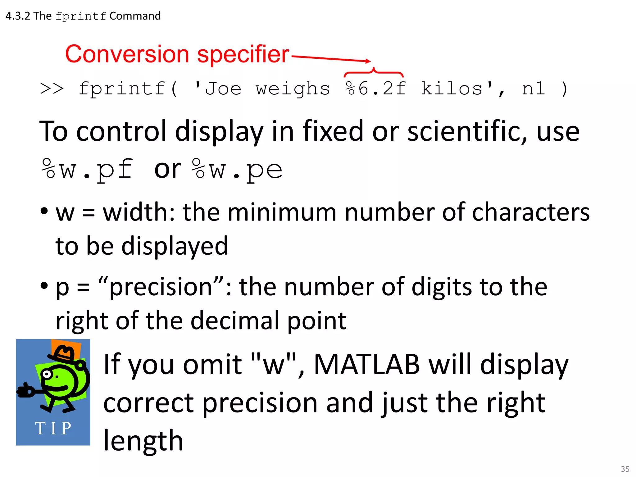
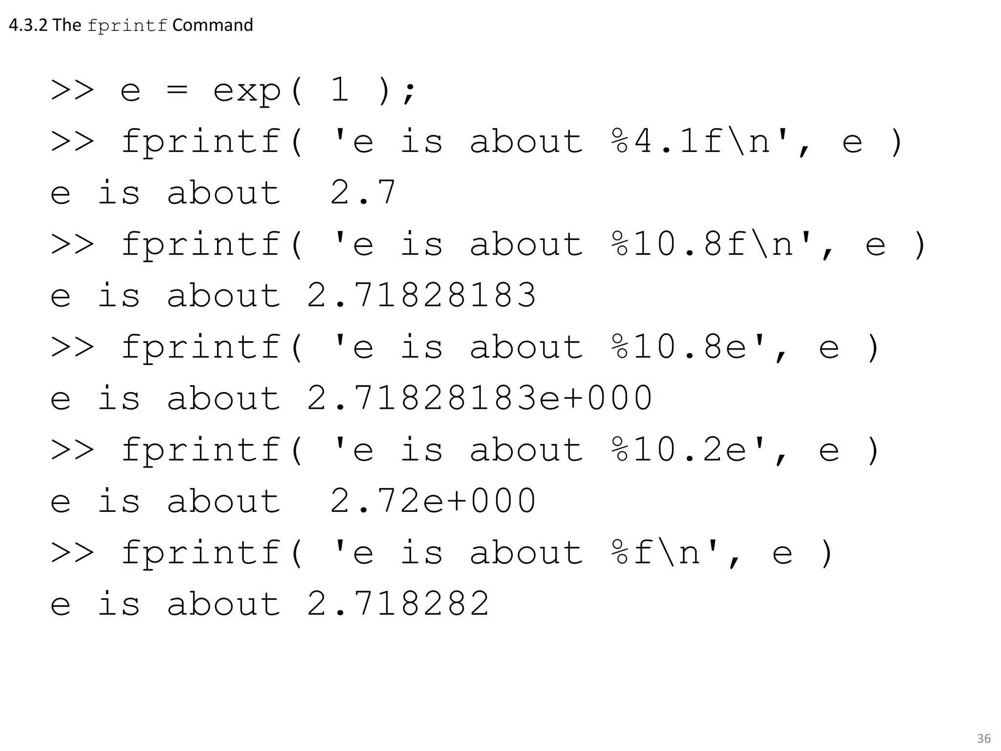
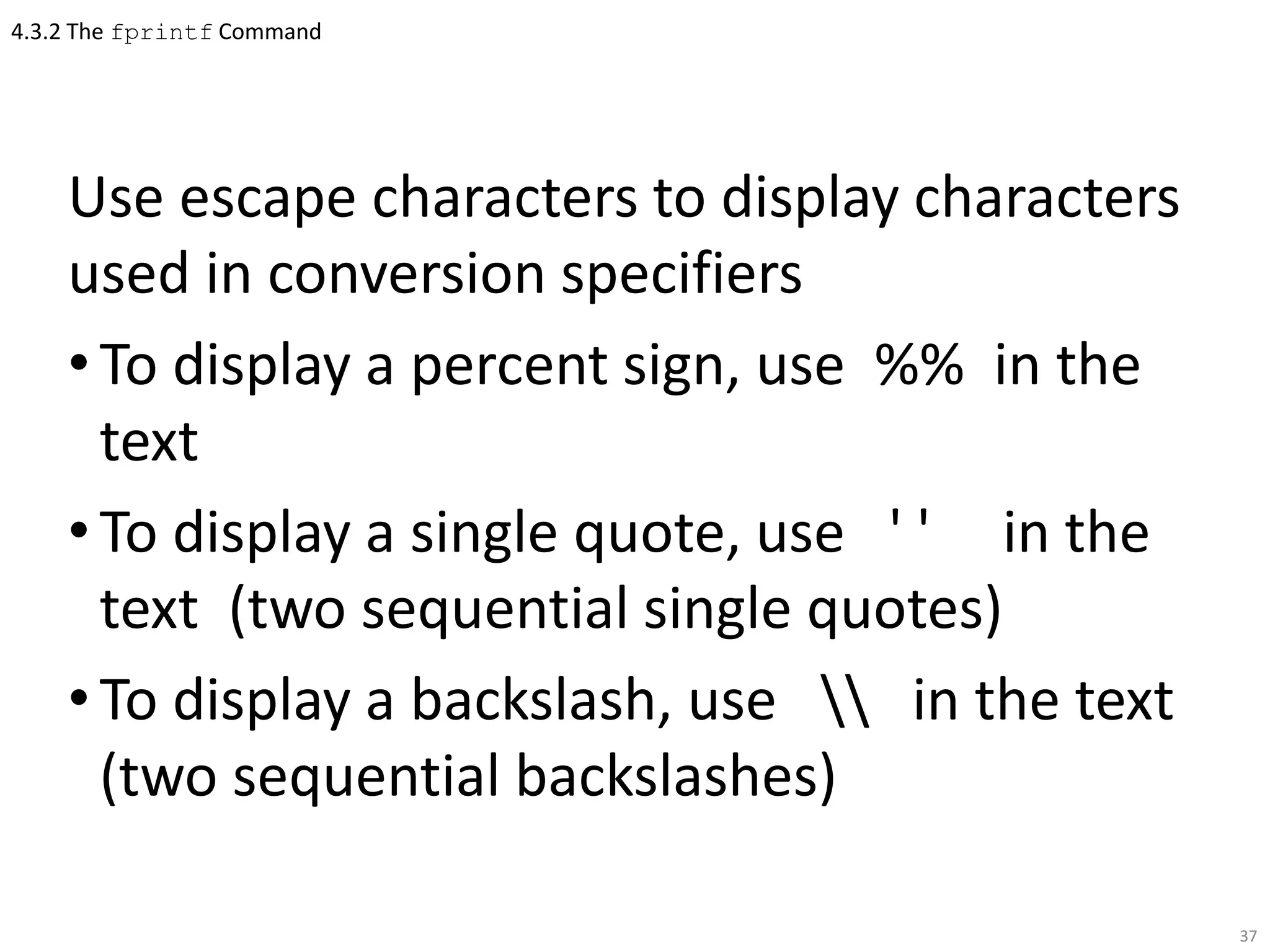
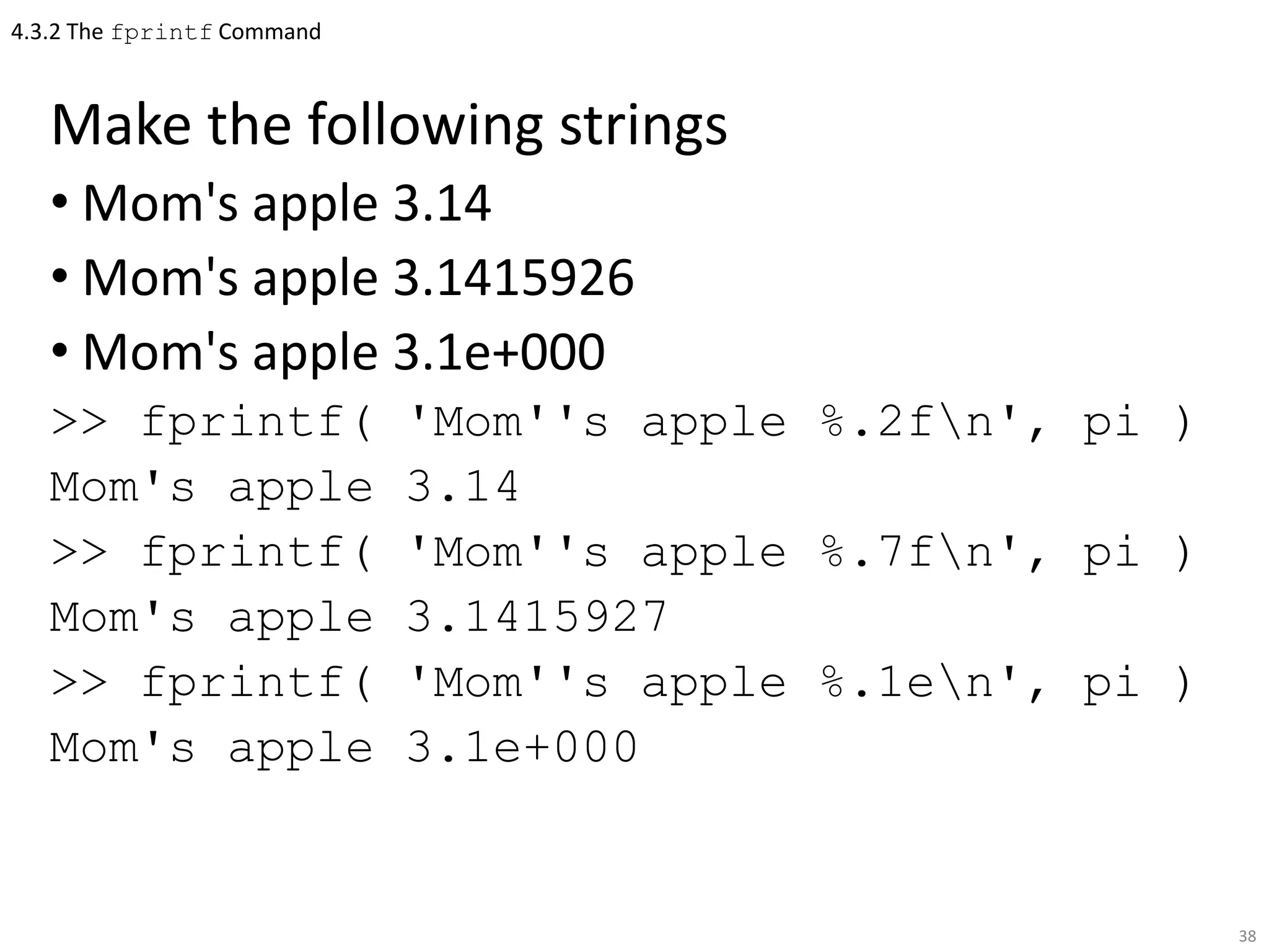
Lesson 19: Double Integrals over General RegionsMatthew Leingang
The document is notes from a math class on double integrals over general regions. It includes announcements about office hours and problem sessions. It defines double integrals over general regions as limits of integrals over unions of rectangles approximating the region. It discusses properties of double integrals and iterated integrals over curved regions of Type I and Type II. It provides examples and worksheets for students to practice evaluating double integrals.
This document contains multiple choice questions related to numerical methods. The questions cover topics like regular falsi method, Newton-Raphson method, numerical integration techniques like trapezoidal rule and Simpson's rule, and numerical differentiation techniques like forward and backward difference formulas. Numerical methods for solving differential equations like Euler's method and Runge-Kutta methods are also addressed.
This document discusses sequences and their limits. Some key points:
- A sequence is a list of numbers written in a definite order. It can be thought of as a function with domain the positive integers.
- The limit of a sequence is defined as the number L such that the terms of the sequence can be made arbitrarily close to L by choosing a sufficiently large term.
- A sequence converges if it has a finite limit, and diverges if its terms approach infinity. Bounded monotonic sequences are guaranteed to converge.
- Properties of sequence limits parallel those of limits of functions, including laws of limits and the ability to pass limits inside continuous functions.
formulation of first order linear and nonlinear 2nd order differential equationMahaswari Jogia
• Equations which are composed of an unknown function and its derivatives are called differential equations.
• Differential equations play a fundamental role in engineering because many physical phenomena are best formulated mathematically in terms of their rate of change.
• When a function involves one dependent variable, the equation is called an ordinary differential equation (ODE).
• A partial differential equation (PDE) involves two or more independent variables.
Figure 1: CHARACTERIZATION OF DIFFERENTIAL EQUATION
FIRST ORDER DIFFERENTIAL EQUATION:
FIRST ORDER LINEAR AND NON LINEAR EQUATION:
A first order equation includes a first derivative as its highest derivative.
- Linear 1st order ODE:
Where P and Q are functions of x.
TYPES OF LINEAR DIFFERENTIAL EQUATION:
1. Separable Variable
2. Homogeneous Equation
3. Exact Equation
4. Linear Equation
i. SEPARABLE VARIABLE:
The first-order differential equation:
Is called separable provided that f(x,y) can be written as the product of a function of x and a function of y.
Suppose we can write the above equation as
We then say we have “separated” the variables. By taking h(y) to the LHS, the equation becomes:
Integrating, we get the solution as:
Where c is an arbitrary constant.
EXAMPLE 1.
Consider the DE :
Separating the variables, we get
Integrating we get the solution as:
This document discusses the divergence of a vector field and the divergence theorem. It begins by defining the divergence of a vector field as a measure of how much that field diverges from a given point. It then illustrates the divergence of a vector field can be positive, negative, or zero at a point. The document expresses the divergence in Cartesian, cylindrical, and spherical coordinate systems. It proves the divergence theorem, which states that the outward flux of a vector field through a closed surface is equal to the volume integral of the divergence of the field over the enclosed volume. The document provides two examples applying the divergence theorem to calculate outward fluxes.
This document provides an overview of numerical differentiation and integration methods. It discusses Newton's forward and backward difference formulas for computing derivatives, as well as Newton-Cote's formula, the trapezoidal rule, and Simpson's one-third and three-eighths rules for numerical integration. Examples of applying these methods to real-world problems are provided. The document also compares Simpson's one-third and three-eighths rules, noting their different assumptions about the polynomial order of the integrated function and requirements for the number of intervals.
Numerical methods and analysis problems/Examplesshehzad hussain
This document describes using the Gauss-Seidel method to solve a system of quadratic equations to estimate the amount of nickel in the organic phase of a liquid-liquid extraction process given experimental data. Initially, the method converges slowly with errors over 50%. Rearranging the equations to make the coefficient matrix more diagonally dominant improves convergence, with errors dropping below 5% after 6 iterations.
The document discusses sequences and series. It defines what a sequence is, including the general term and different types of sequences such as arithmetic, finite, infinite, monotone, and piecewise sequences. It also defines arithmetic sequences specifically and provides the general term for an arithmetic sequence as an = a1 + (n - 1)d, where d is the common difference. Examples are given throughout to illustrate sequence concepts and properties.
The document presents information about differential equations including:
- A definition of a differential equation as an equation containing the derivative of one or more variables.
- Classification of differential equations by type (ordinary vs. partial), order, and linearity.
- Methods for solving different types of differential equations such as variable separable form, homogeneous equations, exact equations, and linear equations.
- An example problem demonstrating how to use the cooling rate formula to calculate the time of death based on measured body temperatures.
The document discusses numerical methods for estimating the derivative of a function f(x) at a point x=xi. It introduces three approaches: 1) the forward difference approximation calculates the slope between xi and xi+h, 2) the backward difference approximation calculates the slope between xi-h and xi, and 3) the centered difference approximation calculates the average of the forward and backward slopes. Each method has an error term that approaches zero as h approaches zero.
Differential equation and its order and degreeMdRiyad5
The order of a differential equation is determined by the highest-order derivative; the degree is determined by the highest power on a variable. The higher the order of the differential equation, the more arbitrary constants need to be added to the general solution
The document discusses various concepts related to lists in Python including:
- What lists are and their main properties like being ordered, containing arbitrary objects that can be accessed by index, and being nestable and mutable.
- Common list methods like insert(), remove(), sort(), etc.
- How to define and assign lists, access list elements, and modify lists.
- List slicing and how it allows accessing a subset of list elements.
- Passing lists to functions and how lists are mutable.
- Algorithms for generating prime numbers and sorting lists like selection sort.
- Basic searching algorithms like linear search and binary search and how they work.
- The concept of list
The document discusses vector spaces and related linear algebra concepts. It defines vector spaces and lists the axioms that must be satisfied. Examples of vector spaces include the set of all pairs of real numbers and the space of 2x2 symmetric matrices. The document also discusses subspaces, linear combinations, span, basis, dimension, row space, column space, null space, rank, nullity, and change of basis. It provides examples and explanations of these fundamental linear algebra topics.
This document discusses topics in partial differentiation including:
1) The geometrical meaning of partial derivatives as the slope of the tangent line to a surface.
2) Finding the equation of the tangent plane and normal line to a surface.
3) Taylor's theorem and Maclaurin's theorem for functions with two variables, which can be used to approximate functions and calculate errors.
2D array in C++ language ,define the concept of c++ Two-Dimensional array .with example .and also Accessing Array Components concept.and Processing Two-Dimensional Arrays.
Presentation on Fourier Series
contents are:-
Euler’s Formula
Functions having point of discontinuity
Change of interval
Even and Odd functions
Half Range series
Harmonic analysis
The document discusses various sorting algorithms. It describes how sorting algorithms arrange elements of a list in a certain order. Efficient sorting is important as a subroutine for algorithms that require sorted input, such as search and merge algorithms. Common sorting algorithms covered include insertion sort, selection sort, bubble sort, merge sort, and quicksort. Quicksort is highlighted as an efficient divide and conquer algorithm that recursively partitions elements around a pivot point.
Pascal's triangle is a triangular array of the binomial coefficients that arises from the binomial formulas. It was studied extensively by the French mathematician Blaise Pascal in the 17th century. The binomial theorem states that the expansion of (a + b)^n can be written as the sum of terms involving the binomial coefficients, with the coefficient of each term found using the appropriate entry in Pascal's triangle. Examples are provided of using the binomial theorem to expand expressions like (x + y)^5 and determining coefficients of specific terms in the expansions.
First order linear differential equationNofal Umair
1. A differential equation relates an unknown function and its derivatives, and can be ordinary (involving one variable) or partial (involving partial derivatives).
2. Linear differential equations have dependent variables and derivatives that are of degree one, and coefficients that do not depend on the dependent variable.
3. Common methods for solving first-order linear differential equations include separation of variables, homogeneous equations, and exact equations.
The document defines and describes various graph concepts and data structures used to represent graphs. It defines a graph as a collection of nodes and edges, and distinguishes between directed and undirected graphs. It then describes common graph terminology like adjacent/incident nodes, subgraphs, paths, cycles, connected/strongly connected components, trees, and degrees. Finally, it discusses two common ways to represent graphs - the adjacency matrix and adjacency list representations, noting their storage requirements and ability to add/remove nodes.
The document defines definite integrals and discusses their properties. It states that a definite integral evaluates to a single number by integrating a function over a closed interval from a lower limit to an upper limit. It gives examples of using definite integrals to find areas bounded by curves. The mean value theorem for integrals is also introduced, which states that there is a rectangle between the inscribed and circumscribed rectangles with an area equal to the region under the curve. Exercises are provided on evaluating definite integrals and applying the mean value theorem.
This document presents an overview of sets in discrete mathematics. It defines what a set is, provides examples of how sets can be written, and discusses the history and methods of defining sets. The document also defines and provides examples of types of sets such as empty, finite, infinite, equal, subset, power, universal, disjoint, union, intersection, and complement sets. It further explains Venn diagrams and their history as a way to visualize logical relations between sets.
This document discusses double-ended queues or deques. Deques allow elements to be added or removed from either end. There are two types: input restricted deques where elements can only be inserted at one end but removed from both ends, and output restricted deques where elements can only be removed from one end but inserted from both ends. Deques can function as stacks or queues depending on the insertion and removal ends. The document describes algorithms for common deque operations like insert_front, insert_back, remove_front, and remove_back. It also lists applications of deques like palindrome checking and task scheduling.
The document discusses Fourier series and two of their applications. Fourier series can be used to represent periodic functions as an infinite series of sines and cosines. This allows approximating functions that are not smooth using trigonometric polynomials. Two key applications are representing forced oscillations, where a periodic driving force can be modeled as a Fourier series, and solving the heat equation, where the method of separation of variables results in a Fourier series representation of temperature over space and time.
This document provides an overview of the topics covered in the Numerical Methods course CISE-301. It discusses:
- Numerical methods as algorithms used to obtain numerical solutions to mathematical problems when analytical solutions do not exist or are difficult to obtain.
- Specific topics that will be covered, including solution of nonlinear equations, linear equations, curve fitting, interpolation, numerical integration, differentiation, and ordinary and partial differential equations.
- An introduction to Taylor series and how they can be used to approximate functions, along with examples of Maclaurin series expansions.
- How numerical representations of real numbers like floating point can lead to rounding errors, and the concepts of accuracy and precision in numerical calculations.
How do you calculate the particular integral of linear differential equations?
Learn this and much more by watching this video. Here, we learn how the inverse differential operator is used to find the particular integral of trigonometric, exponential, polynomial and inverse hyperbolic functions. Problems are explained with the relevant formulae.
This is useful for graduate students and engineering students learning Mathematics. For more videos, visit my page
https://www.mathmadeeasy.co/about-4
Subscribe to my channel for more videos.
This chapter covers two-dimensional (2D) plots in MATLAB. It discusses various plot commands like plot, fplot, and errorbar that can be used to create basic and specialized 2D plots. It also describes how to format plots by adding labels, titles, legends, text annotations and grids. Plots with logarithmic and polar axes as well as histograms are demonstrated. The chapter shows how to create multiple plots on the same figure using subplots or in separate figure windows.
Signal Processing Introduction using Fourier TransformsArvind Devaraj
1) The document introduces signal processing by discussing signals, systems, and transforms. It defines signals as functions of time or space and systems as maps that manipulate signals. Transforms represent signals in different domains like frequency to simplify operations.
2) Signals can be represented in the frequency domain using Fourier transforms. This makes operations like filtering easier. Low frequencies represent overall shape while high frequencies are details like noise or edges.
3) Linear and time-invariant systems can be characterized by their impulse response. The output is the convolution of the input and impulse response. Convolution is a mechanism that shapes signals to produce outputs.
This document provides an overview of file input/output in C including opening, reading, writing, and closing files. It discusses sequential and random access of files. Key functions covered include fopen(), fclose(), fgets(), fputs(), fscanf(), fprintf(), fseek(), rewind(), and their usage. Examples and exercises are provided to demonstrate reading/writing contents, formatted and unformatted I/O, and random access in files.
This Presentation is a draft of a summary of "Learn Python The Hard Way" Book which is very helpful for anyone want to learn python from scratch of
For reading the book and do exercises, the book is available for free here: http://learnpythonthehardway.org/book/
Looping in PythonLab8 lecture slides.pptxadihartanto7
This document provides instructions for writing two Python programs - Vowels.py and NumberProperties.py. Vowels.py asks the user to input a string and prints each character on a new line, then counts and prints the number of lowercase vowels. NumberProperties.py uses a while loop to input multiple numbers, calculates their average, minimum, maximum and range, and prints the results. It provides pseudo-code and explanations of the algorithms and control structures needed to solve the problems.
The document discusses Python input and output functions. It describes how the input() function allows user input and converts the input to a string by default. The print() function outputs data to the screen and allows formatting of output. The document also discusses importing modules to reuse code and functions from other files.
MATLAB is a powerful programming language for technical computing. It allows matrix manipulation, plotting of functions and data, implementation of algorithms, creation of user interfaces, and interfacing with programs in other languages. Some key features of MATLAB include its matrix-based data structure, built-in math and engineering functions, programming tools for algorithm development and testing, and integrated development environment. MATLAB also provides tools for debugging and optimizing code performance such as breakpoints, stepping through code, and the profiler.
This document provides a summary of 16 lessons on C programming:
1. The first few lessons cover include files, the main function, and system pause for prompting user input.
2. Later lessons cover printing messages, commenting code, declaring and assigning variables, and variable types.
3. The final lessons demonstrate mathematical operations in C using addition, subtraction, multiplication, division, and modulos and operating on multiple variables.
A program is a sequence of instructions that are run by the processor. To run a program, it must be compiled into binary code and given to the operating system. The OS then gives the code to the processor to execute. Functions allow code to be reused by defining operations and optionally returning values. Strings are sequences of characters that can be manipulated using indexes and methods. Common string methods include upper() and concatenation using +.
A program is a sequence of instructions that are run by the processor. To run a program, it must be compiled into binary code and given to the operating system. The OS then gives the code to the processor to execute. Functions allow code to be reused by defining operations and returning values. Strings are sequences of characters that can be manipulated using indexes and methods. Common string methods include upper() and concatenation using +.
A program is a sequence of instructions that are run by the processor. To run a program, it must be compiled into binary code and given to the operating system. The OS then tells the processor to execute the program. Functions allow code to be reused by defining operations that take in arguments and return values. Strings are sequences of characters that can be accessed by index and manipulated with methods like upper() that return new strings.
A program is a sequence of instructions that are run by the processor. To run a program, it must be compiled into binary code and given to the operating system. The OS then gives the code to the processor to execute. Functions allow code to be reused by defining operations and returning values. Strings are sequences of characters that can be manipulated using indexes and methods. Common string methods include upper() and concatenation using +.
A program is a sequence of instructions that are run by the processor. To run a program, it must be compiled into binary code and given to the operating system. The OS then gives the code to the processor to execute. Functions allow code to be reused by defining operations and returning values. Strings are sequences of characters that can be accessed by index and manipulated with methods like upper() that return new strings.
The document discusses various C programming concepts like algorithms, flowcharts, tokens, data types, operators, functions, and hardware components of a computer. It includes questions and answers on these topics. Key points covered are definition of algorithm and flowchart, different types of tokens in C, differences between while and do-while loops, definition of software and its types, and examples of standard header files.
Code In PythonFile 1 main.pyYou will implement two algorithms t.pdfaishwaryaequipment
Code In Python
File 1: main.py
You will implement two algorithms to find the shortest path in a graph.
1. def dijkstra(G,start_node): Takes an Adjacency Matrix G and the index of the starting
node start_node. Returns the distance array.
2. def floyd(G): Takes an Adjacency Matrix G and returns the distance matrix
The graph you are working on will be give in a file with the following format.
1. Line 1: The number of Nodes in the Graph
2. Lines 2-EOF: Every other line in the file contains an edge
1. First Value is the FROM node
2. Second Value is the TO node
3. Third Value is the weight of the edge
Note: You should store the weights as floats.
The program will have a command line interface. First ask for the file name of the graph to work
with. Then implement 4 text commands.
· dijkstra x - Runs Dijkstra starting at node X. X must be an integer
· floyd - Runs Floyd\'s algorithm
· help - prints this menu
· exit or ctrl-D - Exist the program
You must implement this using only standard python3 libraries. You may not use any outside
libraries. For example, open source graph libraries. Your code must run on tux with just main.py
and the input files. You may not include any other python files.
Example Run 1
File containing graph: input1.txt
Possible Commands are:
dijkstra x - Runs Dijkstra starting at node X. X must be an integer
floyd - Runs Floyd\'s algorithm
help - prints this menu
exit or ctrl-D - Exits the program
Enter command: help
Possible Commands are:
dijkstra x - Runs Dijkstra starting at node X. X must be an integer
floyd - Runs Floyd\'s algorithm
help - prints this menu
exit or ctrl-D - Exits the program
Enter command: dijkstra 0
[0.0, 1.0, 3.0, 5.0, 7.0]
Enter command: exit
Bye
Example Run 2
File containing graph: input1.txt
Possible Commands are:
dijkstra x - Runs Dijkstra starting at node X. X must be an integer
floyd - Runs Floyd\'s algorithm
help - prints this menu
exit or ctrl-D - Exits the program
Enter command: dijkstra 0
[0.0, 1.0, 3.0, 5.0, 7.0]
Enter command: dijkstra 1
[inf, 0.0, 2.0, 4.0, 6.0]
Enter command: dijkstra 2
[inf, 3.0, 0.0, 2.0, 4.0]
Enter command: dijkstra 3
[inf, 1.0, 3.0, 0.0, 7.0]
Enter command: dijkstra 4
[inf, 6.0, 8.0, 5.0, 0.0]
Enter command: exit
Bye
Example Run 3
File containing graph: input1.txt
Possible Commands are:
dijkstra x - Runs Dijkstra starting at node X. X must be an integer
floyd - Runs Floyd\'s algorithm
help - prints this menu
exit or ctrl-D - Exits the program
Enter command: floyd
[0.0, 1.0, 3.0, 5.0, 7.0]
[inf, 0.0, 2.0, 4.0, 6.0]
[inf, 3.0, 0.0, 2.0, 4.0]
[inf, 1.0, 3.0, 0.0, 7.0]
[inf, 6.0, 8.0, 5.0, 0.0]
Enter command: exit
Bye
Example Run 4
File containing graph: input2.txt
Possible Commands are:
dijkstra x - Runs Dijkstra starting at node X. X must be an integer
floyd - Runs Floyd\'s algorithm
help - prints this menu
exit or ctrl-D - Exits the program
Enter command: dijkstra 0
[0.0, 3.0, 4.0, 4.0, inf, 4.0]
Enter command: dijkstra 1
[inf, 0.0, 1.0, 3.0, inf, 1.0]
Enter command: dijkst.
The document discusses procedural abstraction and functions that return values in programming. It covers topics like top-down design, predefined functions, programmer-defined functions, procedural abstraction, local variables, and overloading function names. Some key points include breaking problems into smaller subtasks using top-down design, how predefined and programmer-defined functions work, the use of return values, and how procedural abstraction hides implementation details through a "black box" approach.
The document discusses the Objective-C preprocessor and underlying C language features. It covers preprocessor directives like #define, #import, #include, and #undef. It also discusses arrays, structures, pointers, functions, and how Objective-C works with C at a low level. Blocks in Objective-C are described as being similar to functions but having some differences like needing to be declared in .m files instead of .h headers.
The document discusses procedural abstraction and functions that return values in programming. It covers the following topics:
- Top-down design for breaking problems into subtasks and functions.
- Predefined functions provided by libraries that perform operations like square roots.
- Defining your own functions through declarations that specify parameters and return types, and definitions that implement the function body.
- Calling functions by name and passing arguments.
- Information hiding through procedural abstraction where functions act as "black boxes".
This document discusses functions and procedural abstraction in C++. It covers:
- Top-down design and breaking problems into subtasks that can be implemented as functions
- Predefined and programmer-defined functions, including function declarations and definitions
- Passing arguments to functions by value and type casting
- Designing functions as "black boxes" using procedural abstraction to hide implementation details
- Scope of variables, including local variables within functions versus global variables
This chapter discusses mathematical operations with arrays in MATLAB. It covers topics such as addition, subtraction, multiplication, and division of arrays. Array operations can be performed elementwise or using matrix multiplication. Built-in functions like mean, max, and sort can be used to analyze array properties. Random number generation functions rand, randn and randi are also introduced.
This document discusses creating and manipulating arrays in MATLAB. It covers:
- Creating one-dimensional arrays (vectors) using known values, spacing, or number of elements.
- Creating two-dimensional arrays (matrices) by specifying rows and ensuring each row has the same number of columns.
- Basic array commands like zeros, ones, and eye to create arrays filled with zeros, ones, or an identity matrix.
- Transposing arrays with the ' operator.
- Accessing and assigning values to individual elements or ranges of elements using indexing and colon notation.
- Adding elements to existing arrays by assigning values to undefined indices or appending rows/columns.
This chapter discusses starting MATLAB and working in the command window. It introduces MATLAB windows like the command window, figure window, editor window, etc. It describes how to do basic arithmetic and define scalar variables in MATLAB. Functions for elementary math operations, trigonometric functions, and managing variables are also introduced.
This document discusses programming concepts in MATLAB including conditional statements, loops, and logical operators. It provides examples of how to:
- Use if, elseif, and else conditional statements to execute different sections of code depending on conditions.
- Implement for loops to repeat a block of code a specified number of times.
- Employ logical operators like & (AND), | (OR), and ~ (NOT) to combine relational expressions and conditionally execute code.
- Compare values, arrays, and scalars using relational operators like <, >, ==, ~=, etc. and logical indexing.
The examples demonstrate how to control program flow and selectively run sections of MATLAB code.
The document provides guidance on how to write an effective CV or resume. It defines what a CV and resume are, as well as the key differences between them. It then outlines the main sections that should be included in a CV, such as contact information, career objective, work experience, education, skills, and references. Tips are provided about what information to include under each section and how to structure and format the CV to make it easy for employers to read. The document also discusses different types of CVs, such as chronological, functional, and hybrid CVs, and their advantages and disadvantages.
The document discusses the history and types of black holes. John Michel and Pierre-Simon Laplace first proposed the idea of invisible stars, or black holes, in the late 1790s. Einstein later predicted black holes in his general relativity theory of 1915. There are two main types: miniature black holes created during the Big Bang and supermassive black holes with masses equal to billions of suns. The central singularity is a point of infinite density where physics breaks down, surrounded by the event horizon from within nothing, not even light, can escape.
Do you want Software for your Business? Visit Deuglo
Deuglo has top Software Developers in India. They are experts in software development and help design and create custom Software solutions.
Deuglo follows seven steps methods for delivering their services to their customers. They called it the Software development life cycle process (SDLC).
Requirement — Collecting the Requirements is the first Phase in the SSLC process.
Feasibility Study — after completing the requirement process they move to the design phase.
Design — in this phase, they start designing the software.
Coding — when designing is completed, the developers start coding for the software.
Testing — in this phase when the coding of the software is done the testing team will start testing.
Installation — after completion of testing, the application opens to the live server and launches!
Maintenance — after completing the software development, customers start using the software.
Measures in SQL (SIGMOD 2024, Santiago, Chile)Julian Hyde
SQL has attained widespread adoption, but Business Intelligence tools still use their own higher level languages based upon a multidimensional paradigm. Composable calculations are what is missing from SQL, and we propose a new kind of column, called a measure, that attaches a calculation to a table. Like regular tables, tables with measures are composable and closed when used in queries.
SQL-with-measures has the power, conciseness and reusability of multidimensional languages but retains SQL semantics. Measure invocations can be expanded in place to simple, clear SQL.
To define the evaluation semantics for measures, we introduce context-sensitive expressions (a way to evaluate multidimensional expressions that is consistent with existing SQL semantics), a concept called evaluation context, and several operations for setting and modifying the evaluation context.
A talk at SIGMOD, June 9–15, 2024, Santiago, Chile
Authors: Julian Hyde (Google) and John Fremlin (Google)
https://doi.org/10.1145/3626246.3653374
Introducing Crescat - Event Management Software for Venues, Festivals and Eve...Crescat
Crescat is industry-trusted event management software, built by event professionals for event professionals. Founded in 2017, we have three key products tailored for the live event industry.
Crescat Event for concert promoters and event agencies. Crescat Venue for music venues, conference centers, wedding venues, concert halls and more. And Crescat Festival for festivals, conferences and complex events.
With a wide range of popular features such as event scheduling, shift management, volunteer and crew coordination, artist booking and much more, Crescat is designed for customisation and ease-of-use.
Over 125,000 events have been planned in Crescat and with hundreds of customers of all shapes and sizes, from boutique event agencies through to international concert promoters, Crescat is rigged for success. What's more, we highly value feedback from our users and we are constantly improving our software with updates, new features and improvements.
If you plan events, run a venue or produce festivals and you're looking for ways to make your life easier, then we have a solution for you. Try our software for free or schedule a no-obligation demo with one of our product specialists today at crescat.io
8 Best Automated Android App Testing Tool and Framework in 2024.pdfkalichargn70th171
Regarding mobile operating systems, two major players dominate our thoughts: Android and iPhone. With Android leading the market, software development companies are focused on delivering apps compatible with this OS. Ensuring an app's functionality across various Android devices, OS versions, and hardware specifications is critical, making Android app testing essential.
A Study of Variable-Role-based Feature Enrichment in Neural Models of CodeAftab Hussain
Understanding variable roles in code has been found to be helpful by students
in learning programming -- could variable roles help deep neural models in
performing coding tasks? We do an exploratory study.
- These are slides of the talk given at InteNSE'23: The 1st International Workshop on Interpretability and Robustness in Neural Software Engineering, co-located with the 45th International Conference on Software Engineering, ICSE 2023, Melbourne Australia
Graspan: A Big Data System for Big Code AnalysisAftab Hussain
We built a disk-based parallel graph system, Graspan, that uses a novel edge-pair centric computation model to compute dynamic transitive closures on very large program graphs.
We implement context-sensitive pointer/alias and dataflow analyses on Graspan. An evaluation of these analyses on large codebases such as Linux shows that their Graspan implementations scale to millions of lines of code and are much simpler than their original implementations.
These analyses were used to augment the existing checkers; these augmented checkers found 132 new NULL pointer bugs and 1308 unnecessary NULL tests in Linux 4.4.0-rc5, PostgreSQL 8.3.9, and Apache httpd 2.2.18.
- Accepted in ASPLOS ‘17, Xi’an, China.
- Featured in the tutorial, Systemized Program Analyses: A Big Data Perspective on Static Analysis Scalability, ASPLOS ‘17.
- Invited for presentation at SoCal PLS ‘16.
- Invited for poster presentation at PLDI SRC ‘16.
Need for Speed: Removing speed bumps from your Symfony projects ⚡️Łukasz Chruściel
No one wants their application to drag like a car stuck in the slow lane! Yet it’s all too common to encounter bumpy, pothole-filled solutions that slow the speed of any application. Symfony apps are not an exception.
In this talk, I will take you for a spin around the performance racetrack. We’ll explore common pitfalls - those hidden potholes on your application that can cause unexpected slowdowns. Learn how to spot these performance bumps early, and more importantly, how to navigate around them to keep your application running at top speed.
We will focus in particular on tuning your engine at the application level, making the right adjustments to ensure that your system responds like a well-oiled, high-performance race car.
SOCRadar's Aviation Industry Q1 Incident Report is out now!
The aviation industry has always been a prime target for cybercriminals due to its critical infrastructure and high stakes. In the first quarter of 2024, the sector faced an alarming surge in cybersecurity threats, revealing its vulnerabilities and the relentless sophistication of cyber attackers.
SOCRadar’s Aviation Industry, Quarterly Incident Report, provides an in-depth analysis of these threats, detected and examined through our extensive monitoring of hacker forums, Telegram channels, and dark web platforms.
What is Augmented Reality Image Trackingpavan998932
Augmented Reality (AR) Image Tracking is a technology that enables AR applications to recognize and track images in the real world, overlaying digital content onto them. This enhances the user's interaction with their environment by providing additional information and interactive elements directly tied to physical images.
What is Master Data Management by PiLog Groupaymanquadri279
PiLog Group's Master Data Record Manager (MDRM) is a sophisticated enterprise solution designed to ensure data accuracy, consistency, and governance across various business functions. MDRM integrates advanced data management technologies to cleanse, classify, and standardize master data, thereby enhancing data quality and operational efficiency.
Software Engineering, Software Consulting, Tech Lead, Spring Boot, Spring Cloud, Spring Core, Spring JDBC, Spring Transaction, Spring MVC, OpenShift Cloud Platform, Kafka, REST, SOAP, LLD & HLD.
Unveiling the Advantages of Agile Software Development.pdfbrainerhub1
Learn about Agile Software Development's advantages. Simplify your workflow to spur quicker innovation. Jump right in! We have also discussed the advantages.
SMS API Integration in Saudi Arabia| Best SMS API ServiceYara Milbes
Discover the benefits and implementation of SMS API integration in the UAE and Middle East. This comprehensive guide covers the importance of SMS messaging APIs, the advantages of bulk SMS APIs, and real-world case studies. Learn how CEQUENS, a leader in communication solutions, can help your business enhance customer engagement and streamline operations with innovative CPaaS, reliable SMS APIs, and omnichannel solutions, including WhatsApp Business. Perfect for businesses seeking to optimize their communication strategies in the digital age.
UI5con 2024 - Keynote: Latest News about UI5 and it’s EcosystemPeter Muessig
Learn about the latest innovations in and around OpenUI5/SAPUI5: UI5 Tooling, UI5 linter, UI5 Web Components, Web Components Integration, UI5 2.x, UI5 GenAI.
Recording:
https://www.youtube.com/live/MSdGLG2zLy8?si=INxBHTqkwHhxV5Ta&t=0
Neo4j - Product Vision and Knowledge Graphs - GraphSummit ParisNeo4j
Dr. Jesús Barrasa, Head of Solutions Architecture for EMEA, Neo4j
Découvrez les dernières innovations de Neo4j, et notamment les dernières intégrations cloud et les améliorations produits qui font de Neo4j un choix essentiel pour les développeurs qui créent des applications avec des données interconnectées et de l’IA générative.
WhatsApp offers simple, reliable, and private messaging and calling services for free worldwide. With end-to-end encryption, your personal messages and calls are secure, ensuring only you and the recipient can access them. Enjoy voice and video calls to stay connected with loved ones or colleagues. Express yourself using stickers, GIFs, or by sharing moments on Status. WhatsApp Business enables global customer outreach, facilitating sales growth and relationship building through showcasing products and services. Stay connected effortlessly with group chats for planning outings with friends or staying updated on family conversations.
Flutter is a popular open source, cross-platform framework developed by Google. In this webinar we'll explore Flutter and its architecture, delve into the Flutter Embedder and Flutter’s Dart language, discover how to leverage Flutter for embedded device development, learn about Automotive Grade Linux (AGL) and its consortium and understand the rationale behind AGL's choice of Flutter for next-gen IVI systems. Don’t miss this opportunity to discover whether Flutter is right for your project.
1. Chapter 4
Using Script Files and Managing Data
MATLAB An Introduction with Applications, 5th Edition
Dr. Amos Gilat
The Ohio State University
2. 4.0
In this chapter will study
• How to input data into a script file
• How MATLAB stores data
• Ways to display and save data
• How to exchange data between
MATLAB and other programs
2
3. 4.1 The MATLAB Workspace and the Workspace Window
MATLAB workspace made up of
variables that you define and store
during a MATLAB session. It includes
variables
• Defined in the Command Window
• Defined in script files
A script file can access all variables that
you defined in the Command Window
3
4. 4.1 The MATLAB Workspace and the Workspace Window
whos command is like who command
but with more information
4
5. 4.1 The MATLAB Workspace and the Workspace Window
Can also view workspace variables in
the Workspace Window
– To open Workspace Window, click on
Layout icon, then Workspace
5
6. 4.1 The MATLAB Workspace and the Workspace Window
To edit (change) a variable in the
Workspace Window
1. Double-click on variable to get the
Variable Editor Window
2. In that window can modify numbers
6
7. 4.1 The MATLAB Workspace and the Workspace Window
In Variable Editor Window
• To change a character, place cursor to right
of character and press BACKSPACE or to left
and press DELETE
• To delete a number, select it by dragging or
double-clicking, then press DELETE or
BACKSPACE
7
8. 4.1 The MATLAB Workspace and the Workspace Window
To delete a variable from the
Workspace Window
• Select variable by dragging or double-
clicking, then
– Press DELETE or BACKSPACE
or
– Right click and select Delete
• Can also delete a variable from Command
Window with command
>> clear variable_name
e.g.,
>> clear g
8
9. 4.2 Input to a Script File
When MATLAB executes (runs) a
script file, any variables used in file
must already have values assigned to
them, i.e., the variables must already
be in the workspace
Can assign a value to a variable in
three ways
9
10. 4.2 Input to a Script File
1. Assign value in script file
• Assignment statement is part of script
• To use different value, must edit file,
save file, and run file again
Note – when variable value (a
number) is part of script, value is said
to be hard-coded
10
12. 4.2 Input to a Script File
2. Assign value in Command Window
• Define variable and assign its value in Command
Window
– From before, know that script file will recognize
variable
• To use different value, assign new value in
Command Window and run file again
– Don't need to resave file
Instead of retyping entire command, use
up-arrow to recall command and then edit
it
12
T I P
15. 4.2 Input to a Script File
3. Assign by prompt in script file
• Script file prompts (asks) user to
enter a value, then script assigns
that value to a variable
Use MATLAB input command to
ask for and get value from user
15
16. 4.2 Input to a Script File
variable_name=input('prompt')
prompt is text that input command
displays in Command Window
• You must put text between single quotes
16
17. 4.2 Input to a Script File
variable_name=input('prompt')
When script executes input command
1. Displays prompt text in Command Window
2. Puts cursor immediately to right of prompt
3. User types value and presses ENTER
4. Script assigns user's value to variable and
displays value unless input command had
semicolon at end
17
18. 4.2 Input to a Script File
Script output (in Command Window)
18
19. 4.2 Input to a Script File
It's helpful to put a space, or a colon
and a space, at the end of the
prompt so that the user's entry is
separated from the prompt.
Example script file:
age = input('Age in 2012');
age = input('Age in 2012 ');
age = input('Age in 2012: ');
19
T I P
20. 4.2 Input to a Script File
Output of script shown with value of
"30" that user entered
Age in 201230
Age in 2012 30
Age in 2012: 30
20
T I P bad
better
good
21. 4.2 Input to a Script File
Can also prompt for and assign a text string
to a variable.
Method 1
Use input as before but user must type in
beginning and ending quote marks
>> name = input( 'Your name: ' )
Your name: 'Joe'
name =
Joe
21
User must type quotes
22. 4.2 Input to a Script File
Method 2
Pass 's' as second argument to input. User
should not enter quotes
variable_name=input('prompt', 's')
>> name=input('Your name: ', 's')
Your name: Joe
name =
Joe
22
User enters without quotes
23. 4.3 Output Commands
When omit semicolon at end of
statement, MATLAB displays result on
screen. You have no control over
appearance of result, e.g., how many
lines, what precision in numbers. Can
use MATLAB command disp for some
control of appearance and fprintf
for full control
23
24. 4.3.1 The disp Command
disp (display) command displays
variable values or text on screen
• Displays each time on new line
• Doesn't print variable name
disp(variable_name) or
disp('text string')
24
25. 4.3.1 The disp Command
Can display tables with headers using
disp
• Clumsy because no control of
column width – must adjust
headers by inserting blanks
• Better to use fprintf
25
26. 4.3.2 The fprintf Command
fprintf
• Means file print formatted
– formatted text is text that can be read by people
– unformatted text looks random to people but
computers can read it
• Can write to screen or to a file
• Can mix numbers and text in output
• Have full control of output display
• Complicated to use
26
27. 4.3.2 The fprintf Command
Using the fprintf command to display text:
Display text with
fprintf('Text to display')
Example
>> fprintf( 'Howdy neighbor' )
Howdy neighbor>>
Problem – Command Window displays
prompt (>>) at end of text, not at start of
next line!
27
Yikes!
28. 4.3.2 The fprintf Command
To make the next thing that MATLAB
writes (after a use of fprintf)
appear on the start of a new line, put
the two
characters "n" at the end of the
fprintf text
>> fprintf( 'Howdy neighborn' )
Howdy neighbor
>>
28
T I P
29. 4.3.2 The fprintf Command
Can also use n in middle of text to make
MATLAB display remainder of text on next
line
>> fprintf('A mannA plannPanaman')
A man
A plan
A canal
Panama
>>
29
30. 4.3.2 The fprintf Command
n is an escape character, a special
combination of two characters that makes
fprintf do something instead of print
the two characters
n – makes following text come out at
start of next line
t – horizontal tab
There are a few more
30
31. 4.3.2 The fprintf Command
fprintf( format, n1, n2, n3 )
>> fprintf( 'Joe weighs %6.2f kilos', n1 )
31
Format string
Argument
Conversion specifier
32. 4.3.2 The fprintf Command
>> fprintf( 'Joe weighs %6.2f kilos', n1 )
Format string
•May contain text and/or conversion
specifiers
•Must be enclosed in SINGLE quotes, not
double quotes, aka quotation marks (" ")
32
33. 4.3.2 The fprintf Command
>> fprintf( 'Joe is %d weighs %f kilos', age, weight )
Arguments
•Number of arguments and conversion
specifiers must be the same
•Leftmost conversion specifier formats
leftmost argument, 2nd to left specifier
formats 2nd to left argument, etc.
33
34. 4.3.2 The fprintf Command
>> fprintf( 'Joe weighs %f kilos', n1 )
Common conversion specifiers
–%f fixed point (decimal always between 1's
and 0.1's place,
e.g., 3.14, 56.8
–%e scientific notation, e.g, 2.99e+008
–%d integers (no decimal point shown)
–%s string of characters
34
Conversion specifier
35. 4.3.2 The fprintf Command
>> fprintf( 'Joe weighs %6.2f kilos', n1 )
To control display in fixed or scientific, use
%w.pf or %w.pe
• w = width: the minimum number of characters
to be displayed
• p = “precision”: the number of digits to the
right of the decimal point
If you omit "w", MATLAB will display
correct precision and just the right
length
35
Conversion specifier
T I P
36. 4.3.2 The fprintf Command
>> e = exp( 1 );
>> fprintf( 'e is about %4.1fn', e )
e is about 2.7
>> fprintf( 'e is about %10.8fn', e )
e is about 2.71828183
>> fprintf( 'e is about %10.8e', e )
e is about 2.71828183e+000
>> fprintf( 'e is about %10.2e', e )
e is about 2.72e+000
>> fprintf( 'e is about %fn', e )
e is about 2.718282
36
37. 4.3.2 The fprintf Command
Use escape characters to display characters
used in conversion specifiers
•To display a percent sign, use %% in the
text
•To display a single quote, use ' ' in the
text (two sequential single quotes)
•To display a backslash, use in the text
(two sequential backslashes)
37
38. 4.3.2 The fprintf Command
Make the following strings
• Mom's apple 3.14
• Mom's apple 3.1415926
• Mom's apple 3.1e+000
>> fprintf( 'Mom''s apple %.2fn', pi )
Mom's apple 3.14
>> fprintf( 'Mom''s apple %.7fn', pi )
Mom's apple 3.1415927
>> fprintf( 'Mom''s apple %.1en', pi )
Mom's apple 3.1e+000
38
39. 4.3.2 The fprintf Command
Format strings are often long. Can break a
string by
1. Put an open square bracket ( [ ) in front of first single quote
2. Put a second single quote where you want to stop the line
3. Follow that quote with an ellipsis (three periods)
4. Press ENTER, which moves cursor to next line
5. Type in remaining text in single quotes
6. Put a close square bracket ( ] )
7. Put in the rest of the fprintf command
39
40. 4.3.2 The fprintf Command
Example
>> weight = 178.3;
>> age = 17;
>> fprintf( ['Tim weighs %.1f lbs'...
' and is %d years old'], weight, age )
Tim weighs 178.3 lbs and is 17 years old
40
41. 4.3.2 The fprintf Command
fprintf is vectorized, i.e., when vector
or matrix in arguments, command repeats
until all elements displayed
• Uses matrix data column by column
41
43. 4.3.2 The fprintf Command
Using the fprintf command to save output to a file:
Takes three steps to write to a file
Step a: – open file
fid=fopen('file_name','permission')
fid – file identifier, lets fprintf know
what file to write its output in
permission – tells how file will be used,
e.g., for reading, writing, both, etc.
43
44. 4.3.2 The fprintf Command
Some common permissions
• r - open file for reading
• w - open file for writing. If file exists, content
deleted. If file doesn't exist, new file created
• a - same as w except if file exists the written data is
appended to the end of the file
• If no permission code specified, fopen uses r
See Help on fopen for all permission
codes
44
45. 4.3.2 The fprintf Command
Step b:
Write to file with fprintf. Use it exactly
as before but insert fid before the format
string, i.e.,
fprintf(fid,'format string',variables)
The passed fid is how fprintf knows to
write to the file instead of display on the
screen
45
46. 4.3.2 The fprintf Command
Step c:
When you're done writing to the file, close it
with the command fclose(fid)
• Once you close it, you can't use that fid
anymore until you get a new one by calling
fopen
Make sure to close every file you open.
Too many open files makes problems for
MATLAB
46
47. 4.3.2 The fprintf Command
Miscellaneous
• If the file name you give to fopen has no path,
MATLAB writes it to the current directory, also
called the working directory
• You can have multiple files open simultaneously
and use fprintf to write to all of them just by
passing it different fids
• You can read the files you make with fprintf
in any text editor, e.g., MATLAB's Editor window
or Notepad
47
48. 4.4 The save and load Commands
Use save command to save workspace
or data
Use load command to retrieve stored
workspace or data
Can use both to exchange data with
non-MATLAB programs
48
49. 4.4.1 The save Command
Use save command to save some or
all workspace variables to hard drive
Two forms
save file_name
save('file_name')
Either one saves all workspace variables,
including their name, type, size, value
49
50. 4.4.1 The save Command
To only save specific variables, list variables
after file name. For example, to save two
variables named var1 and var2
save file_name var1 var2
save('file_name','var1','var2')
50
51. 4.4.1 The save Command
All forms store variables in file called
"file_name.mat"
• Called "mat" file
• Unformatted (binary) file
– Only MATLAB can read mat file, not other
programs
– Can't read file in text editor, or MATLAB Editor
Window
51
52. 4.4.1 The save Command
To save as formatted text (also called
ASCII text)
save file_name –ascii
IMPORTANT – only saves values of variables,
no other info, even their names!
• Can also just save certain variables, as
before
• Usually just use to save value of one
variable
52
53. 4.4.2 The load Command
To load data in a mat file into workspace
load file_name
load( 'file_name')
To load only specific variables from mat
file, e.g., var1 and var2
load file_name var1 var2
load('file_name','var1','var2')
• If variable already exists in workspace, it is
overwritten (its value is replaced by value
in file)
53
54. 4.4.2 The load Command
To load data in a text file into workspace
load file_name
variable = load( 'file_name')
• In first form, creates variable called
file_name and stores all file data in it
• If all rows in file don't have same number of
columns, MATLAB displays an error
• Even if data created from multiple variables all
with same number of columns, load still reads
all data into one variable
– Not very useful in this case
54
55. 4.5 Importing and Exporting Data
• MATLAB often used to analyze data
collected by other programs
• Sometimes need to transfer MATLAB
data to other programs
• In this section will only discuss
numerical data
– MATLAB has commands to load and save
data from a number of other programs
– Can also tell MATLAB what format data is
in
55
56. 4.5.1 Commands for Importing and Exporting Data
Will illustrate transferring data with a
specific program by discussing
Microsoft Excel
• Commonly used to store data
• Works with many programs that
gathers data
• Used often by people with technical
data but for which MATLAB is overkill
56
57. 4.5.1 Commands for Importing and Exporting Data
Importing and exporting data into and from Excel:
Import (read) data from Excel with
variable_name=xlsread('filename')
• Stores all data in one variable
• If Excel file has multiple sheets, reads first
one
– To read from other sheets, pass command
the sheet name
• Can read rectangular section of sheet by
specifying range in command
57
58. 4.5.1 Commands for Importing and Exporting Data
Export (write) data to Excel file with
xlswrite('filename',variable_name)
• Can specify in command name of sheet and
range to write to
58
59. 4.5.2 Using the Import Wizard
MATLAB's import wizard is semi-
automatic way to read data from any
file
• Wizard shows what it thinks format is
• User can then adjust format
Two ways to start Import Wizard
1. In MATLAB desktop,
click Import Data icon
2. With command uiimport
59
60. 4.5.2 Using the Import Wizard
First Wizard display
• Wizard displays file-selection dialog box
• User picks file
• Wizard shows some of data as it is in file and as
how Wizard interprets it
– User can change column separator or number of text
header lines (that Wizard will not try to read)
60
61. 4.5.2 Using the Import Wizard
Second Wizard display
• Shows name and size of variable it will create
• When user selects Finish, Wizard creates that
variable in workspace
– Variable name is file name
61