1
MATLAB An Introduction with Applications, 5th Edition
Dr. Amos Gilat
The Ohio State University
Chapter 3
Mathematical Operations with Arrays
3.0
Previously dealt with scalars (single
numbers). Will now work with
arrays, which in general have more
than one number
This chapter covers basics of using
arrays
2
3.0
array – a rectangular arrangement of
numbers with one or more dimensions
vector – an array with only one column
or one row
scalar – an array with exactly one row
and one column, i.e., a single number
Note – "matrix" and "array" are often
used synonymously
3
3.1 Addition and Subtraction
• Use + to add two arrays or to add a scalar to
an array
• Use – to subtract one array from another or
to subtract a scalar from an array
– When using two arrays, they must both have
the same dimensions (number of rows and
number of columns)
– Vectors must have the same dimensions (rows
and columns), not just the same number of
elements
4
3.1 Addition and Subtraction
When adding two arrays A and B,
MATLAB adds the corresponding
elements, i.e.,
• It adds the element in the first row and
first column of A to the element in the first
row and column of B
• It adds the element in the first row and
second column of A to the element in the
first row and second column of B, etc.
This called elementwise addition
5
3.1 Addition and Subtraction
When subtracting two arrays
A and B, MATLAB performs an
elementwise subtraction
In general, an operation between
two arrays that works on
corresponding elements is called
an elementwise operation
6
3.1 Addition and Subtraction
EXAMPLE
For 𝐴 =
𝐴11 𝐴12 𝐴13
𝐴21 𝐴22 𝐴23
and 𝐵 =
𝐵11 𝐵12 𝐵13
𝐵21 𝐵22 𝐵23
𝐴 + 𝐵 =
𝐴11 + 𝐵11 𝐴12 + 𝐵12 𝐴13 + 𝐵13
𝐴21 + 𝐵21 𝐴22 + 𝐵22 𝐴23 + 𝐵23
𝐴 − 𝐵 =
𝐴11 − 𝐵11 𝐴12 − 𝐵12 𝐴13 − 𝐵13
𝐴21 − 𝐵21 𝐴22 − 𝐵22 𝐴23 − 𝐵23
7
3.1 Addition and Subtraction
When adding a scalar to an array,
MATLAB adds the scalar to every
element of the array
When subtracting a scalar from an
array, MATLAB subtracts the scalar
from every element of the array
8
3.1 Addition and Subtraction
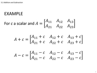
EXAMPLE
For c a scalar and 𝐴 =
𝐴11 𝐴12 𝐴13
𝐴21 𝐴22 𝐴23
𝐴 + 𝑐 =
𝐴11 + 𝑐 𝐴12 + 𝑐 𝐴13 + 𝑐
𝐴21 + 𝑐 𝐴22 + 𝑐 𝐴23 + 𝑐
𝐴 − 𝑐 =
𝐴11 − 𝑐 𝐴12 − 𝑐 𝐴13 − 𝑐
𝐴21 − 𝑐 𝐴22 − 𝑐 𝐴23 − 𝑐
9
3.2 Array Multiplication
There are two ways of multiplying
matrices – matrix multiplication and
elementwise multiplication
MATRIX MULTIPLICATION
• Type used in linear algebra
• MATLAB denotes this with asterisk (*)
• Number of columns in left matrix must be
same as number of rows in right matrix
10
3.2 Array Multiplication
11
3.2 Array Multiplication
12
3.2 Array Multiplication
When performing matrix multiplication
on two square matrices
• They must both have the same dimensions
• The result is a matrix of the same dimension
• In general, the product is not commutative,
i.e., 𝐴 ∗ 𝐵 ≠ 𝐵 ∗ 𝐴
13
3.2 Array Multiplication
>> A = randi(3,3)
A =
3 3 1
3 2 2
1 1 3
>> B=randi(3,3)
B =
3 3 1
1 2 2
3 3 3
>> AB = A*B
AB =
15 18 12
17 19 13
13 14 12
14
>> BA = B*A
BA =
19 16 12
11 9 11
21 18 18
>> AB == BA
ans =
0 0 1
0 0 0
0 0 0
3.2 Array Multiplication
When performing matrix multiplication
on two vectors
• They must both be the same size
• One must be a row vector and the other a
column vector
• If the row vector is on the left, the product is
a scalar
• If the row vector is on the right, the product
is a square matrix whose side is the same
size as the vectors
15
3.2 Array Multiplication
>> h = [ 2 4 6 ]
h =
2 4 6
>> v = [ -1 0 1 ]'
v =
-1
0
1
16
>> h * v
ans =
4
>> v * h
ans =
-2 -4 -6
0 0 0
2 4 6
3.2 Array Multiplication
dot(a,b) computes
inner (dot) product
• a and b must be same size
• Any combination of vertical
or horizontal vectors
• Result is always a scalar
17
EXAMPLE
>> h = [ 2 4 6 ]
h =
2 4 6
>> v = [ -1 0 1 ]'
v =
-1
0
1
>> dot(h,v)
ans =
4
>> dot(v,h)
ans =
4
3.3 Array Division
Identity matrix
• Square matrix with ones on main diagonal
and zeros elsewhere
• When do matrix multiplication on any array
or vector with the identity matrix, array or
vector is unchanged
– True whether multiply with identity matrix on
left or on right
• MATLAB command eye(n) makes an n×n
identity matrix
18
3.3 Array Division
Inverse of a matrix:
Matrix B is the inverse of matrix A if
matrix product of A and B is the identity
matrix I
• Both matrices must be square and same
dimensions
• Multiplication can be from either side, i.e.,
𝐵𝐴 = 𝐴𝐵 = 𝐼
EXAMPLE
19
3.3 Array Division
In math, inverse of a matrix A is written
as A-1
In MATLAB, get inverse with A^-1 or
inv(A)
20
3.3 Array Division
Determinants:
A determinant is a function associated
with square matrices
• In math, determinant of A is written as
det(A) or |A|
• In MATLAB, compute determinant of A
with det(A)
• A matrix has an inverse only if it is square
and its determinant is not zero
If you don't remember much about determinants, go back to
your linear algebra book and review them
21
3.3 Array Division
Left division, :
Left division is one of MATLAB's two
kinds of array division
• Used to solve the matrix equation AX=B
– A is a square matrix, X, B are column vectors
– Solution is X = A-1B
In MATLAB, solve by using left division
operator (), i.e.,
>> X = A  B
22
3.3 Array Division
When solving set of linear equations, use
left division, not inverse, i.e., use X=AB
not X=inv(A)*B
Left division is
• 2-3 times faster
• Often produces smaller error than inv()
• Sometimes inv()can produce erroneous
results
23
3.3 Array Division
Right division, /:
Right division is the other kind of
MATLAB's array division
• Used to solve the matrix equation XC=D
– C is a square matrix, X, D are row vectors
– Solution is X = D·C-1
In MATLAB, solve by using right division
operator (/), i.e.,
>> X = D / C
24
3.4 Element-by-Element Operations
Another way of saying elementwise
operations is element-by-element
operations
• Addition and subtraction of arrays is
always elementwise
• Multiplication, division, exponentiation
of arrays can be elementwise
• Both arrays must be same dimension
25
3.4 Element-by-Element Operations
Do elementwise multiplication,
division, exponentiation by putting a
period in front of the arithmetic
operator
26
3.4 Element-by-Element Operations
27
3.4 Element-by-Element Operations
28
3.4 Element-by-Element Operations
ELEMENTWISE MULTIPLICATION
• Use .* to get elementwise multiplication
(notice period before asterisk)
• Both matrices must have the same
dimensions
>> A = [1 2; 3 4];
>> B = [0 1/2; 1 -1/2];
>> C = A .* B
>> C =
0 1
3 -2
29
3.4 Element-by-Element Operations
If matrices not same dimension in
elementwise multiplication, MATLAB gives
error
>> A = [ 1 2; 3 4];
>> B = [1 0]';
>> A .* B % Meant matrix multiplication!
??? Error using ==> times
Matrix dimensions must agree.
>> A * B % this works
ans =
1
3
30
3.4 Element-by-Element Operations
Be careful – when multiplying square
matrices
• Both types of multiplication always work
• If you specify the wrong operator, MATLAB
will do the wrong computation and there
will be no error!
– Difficult to find this kind of mistake
31
3.4 Element-by-Element Operations
EXAMPLE
>> A = [1 2; 3 4];
>> B = [0 1/2; 1 -1/2];
>> A .* B
>> ans
0 1
3 -2
>> A * B
ans =
2.0000 -0.5000
4.0000 -0.5000
32
3.4 Element-by-Element Operations
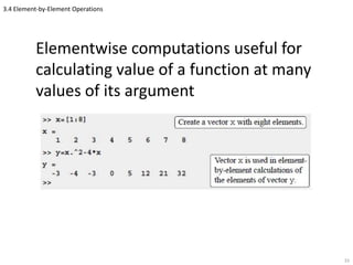
Elementwise computations useful for
calculating value of a function at many
values of its argument
33
3.5 Using Arrays in MATLAB Built-in Functions
Built-in MATLAB functions can accept arrays
as inputs
• When input is array, output is array of same size
with each element being result of function
applied to corresponding input element
– Example: if x is a 7-element row vector, cos(x) is
[cos(x1) cos(x2) cos(x3) cos(x4) cos(x5) cos(x6) cos(x7)]
34
3.6 Built-in Functions for Analyzing Arrays
MATLAB has lots of functions for
operating on arrays. For a vector v
• mean(v) – mean (average)
• max(v) – maximum value, optionally
with index of maximum
• min(v) – minimum value, optionally
with index of minimum
• sum(v) – sum
• sort(v) – elements sorted into
ascending order
35
3.6 Built-in Functions for Analyzing Arrays
• median(v) – median
• std(v) – standard deviation
• dot(v,w) – dot (inner product); v, w both
vectors of same size but any dimension
• cross(v,w) – cross product; v, w must
both have three elements but any dimension
• det(A) – determinant of square matrix A
• inv(A) – inverse of square matrix A
36
3.6 Built-in Functions for Analyzing Arrays
See Table 3-1 for details on the
preceding functions
Note that in all but last four functions
of Table 3-1, A is a vector, not a
matrix. The table does not apply if A is
a matrix
37
3.7 Generation of Random Numbers
Random numbers often used in MATLAB
engineering applications
• Simulate noise
• Useful in certain mathematical
computations, such as Monte Carlo
simulations
38
3.7 Generation of Random Numbers
MATLAB has three commands that
create random numbers – rand,
randn, randi
• All can create scalars, vectors, or
matrices of random numbers
39
3.7 Generation of Random Numbers
rand generates random numbers uniformly
distributed between 0 and 1
• To get numbers between a and b, multiply output of
rand by b-a and add a, i.e., (b-a)*rand + a
See Table 3-2 for some of different ways of
calling rand
40
3.7 Generation of Random Numbers
randi generates uniformly distributed
random integers in a specified range
For example, to make a 3×4 of random
numbers between 50 and 90
>> d=randi( [50 90],3,4)
d =
57 82 71 75
66 52 67 61
84 66 76 67
See Table 3-3 for some of different ways of
calling randi
41
3.7 Generation of Random Numbers
randn generates random numbers from
a normal distribution with mean 0 and
standard deviation 1
Can call randn in same ways as rand,
as Table 3-2 shows
42
3.7 Generation of Random Numbers
To get numbers with mean μ and
standard deviation σ, multiply output of
randn by μ and add σ, i.e.,
sigma * rand + mu
43
3.7 Generation of Random Numbers
To get normally distributed integers
apply the round function to previous
formula, i.e.,
round( sigma * rand + mu )
EXAMPLE
>> w = round(4*randn(1,6)+50)
W =
51 49 46 49 50 44
44

Matlab ch1 (4)

  • 1.
    1 MATLAB An Introductionwith Applications, 5th Edition Dr. Amos Gilat The Ohio State University Chapter 3 Mathematical Operations with Arrays
  • 2.
    3.0 Previously dealt withscalars (single numbers). Will now work with arrays, which in general have more than one number This chapter covers basics of using arrays 2
  • 3.
    3.0 array – arectangular arrangement of numbers with one or more dimensions vector – an array with only one column or one row scalar – an array with exactly one row and one column, i.e., a single number Note – "matrix" and "array" are often used synonymously 3
  • 4.
    3.1 Addition andSubtraction • Use + to add two arrays or to add a scalar to an array • Use – to subtract one array from another or to subtract a scalar from an array – When using two arrays, they must both have the same dimensions (number of rows and number of columns) – Vectors must have the same dimensions (rows and columns), not just the same number of elements 4
  • 5.
    3.1 Addition andSubtraction When adding two arrays A and B, MATLAB adds the corresponding elements, i.e., • It adds the element in the first row and first column of A to the element in the first row and column of B • It adds the element in the first row and second column of A to the element in the first row and second column of B, etc. This called elementwise addition 5
  • 6.
    3.1 Addition andSubtraction When subtracting two arrays A and B, MATLAB performs an elementwise subtraction In general, an operation between two arrays that works on corresponding elements is called an elementwise operation 6
  • 7.
    3.1 Addition andSubtraction EXAMPLE For 𝐴 = 𝐴11 𝐴12 𝐴13 𝐴21 𝐴22 𝐴23 and 𝐵 = 𝐵11 𝐵12 𝐵13 𝐵21 𝐵22 𝐵23 𝐴 + 𝐵 = 𝐴11 + 𝐵11 𝐴12 + 𝐵12 𝐴13 + 𝐵13 𝐴21 + 𝐵21 𝐴22 + 𝐵22 𝐴23 + 𝐵23 𝐴 − 𝐵 = 𝐴11 − 𝐵11 𝐴12 − 𝐵12 𝐴13 − 𝐵13 𝐴21 − 𝐵21 𝐴22 − 𝐵22 𝐴23 − 𝐵23 7
  • 8.
    3.1 Addition andSubtraction When adding a scalar to an array, MATLAB adds the scalar to every element of the array When subtracting a scalar from an array, MATLAB subtracts the scalar from every element of the array 8
  • 9.
    3.1 Addition andSubtraction EXAMPLE For c a scalar and 𝐴 = 𝐴11 𝐴12 𝐴13 𝐴21 𝐴22 𝐴23 𝐴 + 𝑐 = 𝐴11 + 𝑐 𝐴12 + 𝑐 𝐴13 + 𝑐 𝐴21 + 𝑐 𝐴22 + 𝑐 𝐴23 + 𝑐 𝐴 − 𝑐 = 𝐴11 − 𝑐 𝐴12 − 𝑐 𝐴13 − 𝑐 𝐴21 − 𝑐 𝐴22 − 𝑐 𝐴23 − 𝑐 9
  • 10.
    3.2 Array Multiplication Thereare two ways of multiplying matrices – matrix multiplication and elementwise multiplication MATRIX MULTIPLICATION • Type used in linear algebra • MATLAB denotes this with asterisk (*) • Number of columns in left matrix must be same as number of rows in right matrix 10
  • 11.
  • 12.
  • 13.
    3.2 Array Multiplication Whenperforming matrix multiplication on two square matrices • They must both have the same dimensions • The result is a matrix of the same dimension • In general, the product is not commutative, i.e., 𝐴 ∗ 𝐵 ≠ 𝐵 ∗ 𝐴 13
  • 14.
    3.2 Array Multiplication >>A = randi(3,3) A = 3 3 1 3 2 2 1 1 3 >> B=randi(3,3) B = 3 3 1 1 2 2 3 3 3 >> AB = A*B AB = 15 18 12 17 19 13 13 14 12 14 >> BA = B*A BA = 19 16 12 11 9 11 21 18 18 >> AB == BA ans = 0 0 1 0 0 0 0 0 0
  • 15.
    3.2 Array Multiplication Whenperforming matrix multiplication on two vectors • They must both be the same size • One must be a row vector and the other a column vector • If the row vector is on the left, the product is a scalar • If the row vector is on the right, the product is a square matrix whose side is the same size as the vectors 15
  • 16.
    3.2 Array Multiplication >>h = [ 2 4 6 ] h = 2 4 6 >> v = [ -1 0 1 ]' v = -1 0 1 16 >> h * v ans = 4 >> v * h ans = -2 -4 -6 0 0 0 2 4 6
  • 17.
    3.2 Array Multiplication dot(a,b)computes inner (dot) product • a and b must be same size • Any combination of vertical or horizontal vectors • Result is always a scalar 17 EXAMPLE >> h = [ 2 4 6 ] h = 2 4 6 >> v = [ -1 0 1 ]' v = -1 0 1 >> dot(h,v) ans = 4 >> dot(v,h) ans = 4
  • 18.
    3.3 Array Division Identitymatrix • Square matrix with ones on main diagonal and zeros elsewhere • When do matrix multiplication on any array or vector with the identity matrix, array or vector is unchanged – True whether multiply with identity matrix on left or on right • MATLAB command eye(n) makes an n×n identity matrix 18
  • 19.
    3.3 Array Division Inverseof a matrix: Matrix B is the inverse of matrix A if matrix product of A and B is the identity matrix I • Both matrices must be square and same dimensions • Multiplication can be from either side, i.e., 𝐵𝐴 = 𝐴𝐵 = 𝐼 EXAMPLE 19
  • 20.
    3.3 Array Division Inmath, inverse of a matrix A is written as A-1 In MATLAB, get inverse with A^-1 or inv(A) 20
  • 21.
    3.3 Array Division Determinants: Adeterminant is a function associated with square matrices • In math, determinant of A is written as det(A) or |A| • In MATLAB, compute determinant of A with det(A) • A matrix has an inverse only if it is square and its determinant is not zero If you don't remember much about determinants, go back to your linear algebra book and review them 21
  • 22.
    3.3 Array Division Leftdivision, : Left division is one of MATLAB's two kinds of array division • Used to solve the matrix equation AX=B – A is a square matrix, X, B are column vectors – Solution is X = A-1B In MATLAB, solve by using left division operator (), i.e., >> X = A B 22
  • 23.
    3.3 Array Division Whensolving set of linear equations, use left division, not inverse, i.e., use X=AB not X=inv(A)*B Left division is • 2-3 times faster • Often produces smaller error than inv() • Sometimes inv()can produce erroneous results 23
  • 24.
    3.3 Array Division Rightdivision, /: Right division is the other kind of MATLAB's array division • Used to solve the matrix equation XC=D – C is a square matrix, X, D are row vectors – Solution is X = D·C-1 In MATLAB, solve by using right division operator (/), i.e., >> X = D / C 24
  • 25.
    3.4 Element-by-Element Operations Anotherway of saying elementwise operations is element-by-element operations • Addition and subtraction of arrays is always elementwise • Multiplication, division, exponentiation of arrays can be elementwise • Both arrays must be same dimension 25
  • 26.
    3.4 Element-by-Element Operations Doelementwise multiplication, division, exponentiation by putting a period in front of the arithmetic operator 26
  • 27.
  • 28.
  • 29.
    3.4 Element-by-Element Operations ELEMENTWISEMULTIPLICATION • Use .* to get elementwise multiplication (notice period before asterisk) • Both matrices must have the same dimensions >> A = [1 2; 3 4]; >> B = [0 1/2; 1 -1/2]; >> C = A .* B >> C = 0 1 3 -2 29
  • 30.
    3.4 Element-by-Element Operations Ifmatrices not same dimension in elementwise multiplication, MATLAB gives error >> A = [ 1 2; 3 4]; >> B = [1 0]'; >> A .* B % Meant matrix multiplication! ??? Error using ==> times Matrix dimensions must agree. >> A * B % this works ans = 1 3 30
  • 31.
    3.4 Element-by-Element Operations Becareful – when multiplying square matrices • Both types of multiplication always work • If you specify the wrong operator, MATLAB will do the wrong computation and there will be no error! – Difficult to find this kind of mistake 31
  • 32.
    3.4 Element-by-Element Operations EXAMPLE >>A = [1 2; 3 4]; >> B = [0 1/2; 1 -1/2]; >> A .* B >> ans 0 1 3 -2 >> A * B ans = 2.0000 -0.5000 4.0000 -0.5000 32
  • 33.
    3.4 Element-by-Element Operations Elementwisecomputations useful for calculating value of a function at many values of its argument 33
  • 34.
    3.5 Using Arraysin MATLAB Built-in Functions Built-in MATLAB functions can accept arrays as inputs • When input is array, output is array of same size with each element being result of function applied to corresponding input element – Example: if x is a 7-element row vector, cos(x) is [cos(x1) cos(x2) cos(x3) cos(x4) cos(x5) cos(x6) cos(x7)] 34
  • 35.
    3.6 Built-in Functionsfor Analyzing Arrays MATLAB has lots of functions for operating on arrays. For a vector v • mean(v) – mean (average) • max(v) – maximum value, optionally with index of maximum • min(v) – minimum value, optionally with index of minimum • sum(v) – sum • sort(v) – elements sorted into ascending order 35
  • 36.
    3.6 Built-in Functionsfor Analyzing Arrays • median(v) – median • std(v) – standard deviation • dot(v,w) – dot (inner product); v, w both vectors of same size but any dimension • cross(v,w) – cross product; v, w must both have three elements but any dimension • det(A) – determinant of square matrix A • inv(A) – inverse of square matrix A 36
  • 37.
    3.6 Built-in Functionsfor Analyzing Arrays See Table 3-1 for details on the preceding functions Note that in all but last four functions of Table 3-1, A is a vector, not a matrix. The table does not apply if A is a matrix 37
  • 38.
    3.7 Generation ofRandom Numbers Random numbers often used in MATLAB engineering applications • Simulate noise • Useful in certain mathematical computations, such as Monte Carlo simulations 38
  • 39.
    3.7 Generation ofRandom Numbers MATLAB has three commands that create random numbers – rand, randn, randi • All can create scalars, vectors, or matrices of random numbers 39
  • 40.
    3.7 Generation ofRandom Numbers rand generates random numbers uniformly distributed between 0 and 1 • To get numbers between a and b, multiply output of rand by b-a and add a, i.e., (b-a)*rand + a See Table 3-2 for some of different ways of calling rand 40
  • 41.
    3.7 Generation ofRandom Numbers randi generates uniformly distributed random integers in a specified range For example, to make a 3×4 of random numbers between 50 and 90 >> d=randi( [50 90],3,4) d = 57 82 71 75 66 52 67 61 84 66 76 67 See Table 3-3 for some of different ways of calling randi 41
  • 42.
    3.7 Generation ofRandom Numbers randn generates random numbers from a normal distribution with mean 0 and standard deviation 1 Can call randn in same ways as rand, as Table 3-2 shows 42
  • 43.
    3.7 Generation ofRandom Numbers To get numbers with mean μ and standard deviation σ, multiply output of randn by μ and add σ, i.e., sigma * rand + mu 43
  • 44.
    3.7 Generation ofRandom Numbers To get normally distributed integers apply the round function to previous formula, i.e., round( sigma * rand + mu ) EXAMPLE >> w = round(4*randn(1,6)+50) W = 51 49 46 49 50 44 44