Structural-Dynamics

1. 28/08/2025
1
Structural Dynamics

2. Degrees of Freedom:
The number of independent displacement
coordinates required to define the displaced
positions of all the masses relative to their original
position is called the number of Degrees of
Freedom of the system.
Structural Dynamics:
When there are change of inertia and the forces
acting on the structure with respect to time, then
we call it a Dynamic problem.

3. x
y
O
Equation of motion:
Taking moments about point O,
sin 0
I mgL
 
 

Degree of freedom:
Coordinates x and y are related
as the string length L is fixed. So
it has Single degree of freedom
2 2 2
( , , ) 0
x y L
f x y t
 
 
When the constraint equation can
be expressed in this form, then
the system is called Holonomic
system.
Simple pendulum

4. SDOF system
k
c
( )
x t
m
( )
f t
( )
x t
( )
f t
m
Assumptions
• Beam is rigid flexurally and having no ration but lateral
deformation only.
• Columns are massless.
• Mass of the system is ‘m’, stiffness is ‘k’, and damping coefficient is
‘c’, which is defined as the force required to induce unit velocity in
the system.

5. D’ Alembert’s Principle:
Sum of the difference between forces acting on a system of particles
and the time derivative of the momentum projected onto a virtual
displacement consistent with the constraint is zero.
Which can be expressed as:
SDOF system
k
c
( )
x t
m
( )
f t
( )
x t
( )
f t
m
( ) 0
i
i i r
i
d
F m v
dt
  


6. Dynamic equilibrium equation:
Applying D’ Alembert’s principle on the system:
SDOF system
k
c
( )
x t
m
( )
f t
( )
x t
( )
f t
m
( ) 0
, cannot be zero,
( ) 0
( )
i
i
d
r
dt
r
d
dt
F kx cx mx
As
F kx cx mx
mx kx cx F t
    

    
   
 
 
 

7. Free Body Diagram Approach
k
c
( )
x t
m
( )
f t
( )
f t
m
mx

cx

kx
Dynamic equilibrium equation:
Taking summation of all forces in x direction, we get
( )
mx kx cx F t
  
 
For Undamped vibration the dynamic equilibrium equation
will be:
It is a second order linear differential equation of first degree.
( )
mx kx F t
 


8. 28/08/2025
8
Solution of homogenous DE
2
2
1 2
1 2
0
will be a trial solution.
Auxiliary Eqn. will be
0
1
, 4
2
= ,
Case 1, when , are real and distinct,
x(t)=
If a differential equation has the form,
t
x ax bx
x e
a b
or a a b

 

 
 
  
 

  
 
   
 

 
1 2
1 2
1 2
1 2
1 2
c c
Case 2, when , are real and equal,
x(t)=(c c )
Case 3, when , are complex and in the form
(t) [ cos sin ]
t t
t
at
e e
t e
a ib
x e A bt B bt
 

 
 

 

  

9. Undamped Free Vibration
k
c
( )
x t
m
Dynamic equilibrium equation:
0
mx kx
 

2
2
2 2
0
Auxiliary Eqn. will be
0
,
( ) cos sin
, n
n
n
n
n n
k
m
x x
or i
x t A t B t
Let






 

  

 

  


10. Undamped Free Vibration
k
c
( )
x t
m
0
0
;
(0) ;
(0)
x x
x x


 
0
0
0
0
0
0
2 2
0
0
1 0
0
;
( ) cos sin ;
Let, cos ; sin
( ) cos( )
, ( ) Amplitude of motion
tan ( ) Phase Angle
n
n n
n
n
n
n
n
A x
x
and B
x
x t x t t
x
x C and C
x t C t
x
where C x
x
x

 

 

 






  
 
  
  
 





Imposing initial conditions

11. 28/08/2025
11
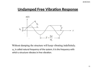
Undamped Free Vibration Response
Without damping the structure will keep vibrating indefinitely.
ωn is called natural frequency of the system, it is the frequency with
which a structure vibrates in free vibration.

12. 28/08/2025
12
Damped Free Vibration
k
c
( )
x t
m
Dynamic equilibrium equation:
0
mx cx kx
  
 
2
2
2 2
2 2
2
0
Auxiliary Eqn. will be
0
( ) 4
,
2
( ) 4
2
, n
n
n
n
k
m
c
x x x
m
c
m
c c
m m
or
c c mk
m
Let
 






   

  

 

  

 

13. 28/08/2025
13
Damped Free Vibration
Case 1.
2
, ( ) 4 0
4
, c 2m n cr
When c mk
c mk
or c

 
 
 
Ccr is called critical damping of the system.
1 2
( )
2
1 2 1 2
2
Solution of the differential equation will be
x(t) =(c ) (c )
cr
n
cr
c
t
t
m
c
m
c t e c t e 
 



  

  
This type of system is called critically damped system.

14. 28/08/2025
14
Imposing initial conditions
Critically Damped systems
0
0
;
(0) ;
(0)
x x
x x


 
1 0
2 0 0
0 0
;
( ) [ (1 ) ]
n
n
t
n
c x
and c x x
x t e x t x t





 
   



15. 28/08/2025
15
Damped Free Vibration
Case 2. 2
, ( ) 4 >0
When c mk

2
2 2 2
2
/
/ 2
/
( ) 4
2
( ) 4
2
2 1
[ Let, ]
2
2
[ Let, 1]
2
=
n
n
cr
d
d n
n d
c c mk
m
c c m
m
c m c
m c
c m
m


 


  
 
  

  

  
 
 
  
 


This type of system is called overdamped system. Where >1


16. 28/08/2025
16
Imposing initial conditions
Overdamped systems
0
0
;
(0) ;
(0)
x x
x x


 
/
0 0
1 /
/
0 0
2 /
( )
2
( )
,
2
n d
d
n d
d
x x
c
x x
and c
 

 

 

   



/ /
1 2
Solution of the differential equation will be
x(t) =e [c e c e ]
n d d
t t t
  
 



17. 28/08/2025
17
Damped Free Vibration
Case 3. 2
, ( ) 4 <0
When c mk

2
2
2
1(4 )
2
2 1
[ Let, ]
2
2
[ Let, 1 ]
2
=
n
cr
d
d n
n d
c mk c
m
c i m c
m c
c i m
m
i

 


  
 
   

  
 
 
  
 


This type of system is called underdamped system. Where <1

ωd is called damped natural frequency of the system.

18. 28/08/2025
18
Imposing initial conditions
Underdamped systems
0
0
;
(0) ;
(0)
x x
x x


 
0
0 0
;
n
d
A x
x x
B






Solution of the differential equation will be
x(t) =e [ cos sin ]
nt
d d
A t B t

 




19. 28/08/2025
19
Logarithmic decrement
k
c
( )
x t
m
1
2
1 1 1 1
2 2 2 2
2 1
1
2
2
1
2
2
Let,
( ) [ cos sin ]
, ( ) [ cos sin ]
if,
2
1
2
ln
1
is called logarithmic decrement.
For very low damping, 2
n
n
n d
t
d d
t
d d
d
T
d d n
d
x t e A t B t
and x t e A t B t
t t T
x
e
x
T and
x
x



 
 

  


 


 


 
 
 
 
  
  




20. 28/08/2025
20
Forced vibration
k
c
( )
x t
m
( )
f t Equation of motion,
, ( ) sin
( )
Let F t P t
mx kx cx F t


  
 
1 2
1 2
. ( ) [ cos sin ]
If the system is excited by a sinusoid, the response will also be a
sinusoid, so for finding P.I let the trial solution be,
( ) cos sin
( ) sin
nt
c d d
p
p
C F x t e A t B t
x t C t C t
x t C t C

 
 
 

  
 
  

2
1 2
cos
( ) ( cos sin )
p
t
x t C t C t
 
  
  


21. 28/08/2025
21
2
2 2
1 2 1
2 2
2 1 2
2 2
1 2 1
2 2
2 1 2
Putting in the equation of motion,
2 sin
We get,
[-C +C .2 +C ]cos t
+ [-C -C .2 +C ]sin t=0
[-C +C .2 +C ] 0.......................(1)
[-C -C .2 +C
n n
n n
n n
n n
n n
P
x x x t
m
P
m
  
    
    
   
   
  

 
 
 
]=0..................(2)
Let, Frequency ratio,
n
P
m
r



Forced vibration

22. 28/08/2025
22
2
1 2
2
1 2 2
1 2 2 2
2
2 2 2 2
1 2
2
2 2 2
We get,
C (1 ) (2 ) 0...............( )
(2 ) (1 ) .....( )
(2 )
(1 ) (2 )
(1 )
(1 ) (2 )
( ) cos sin
1
[(1 )sin (2 )co
(1 ) (2 )
n
p
r C r i
P
C r C r ii
m
P r
C
k r r
P r
C
k r r
x t C t C t
P
r t r
k r r






 
 

  
   

 
 

 
 
  
  
 
2 2 2
2 2 2
s ]
1
sin( )
(1 ) (2 )
1
= sin( )
(1 ) (2 )
st
t
P
t
k r r
x t
r r

 

 

 
 

 

23. 28/08/2025
23
Dynamic amplification factor
DMF:
DMF is the ratio of the dynamic response to static response of a
structure, and is given by
2 2 2
1
(1 ) (2 )
D
r r


 
P
l
a
c
e
f
o
r
g
r
a
p
h
Dynamic Magnification Factor (DMF)

24. 28/08/2025
24
Phase angle
P
l
a
c
e
f
o
r
g
r
a
p
h

25. 28/08/2025
25
Force transmitted to support
k
c
( )
x t
m
( )
f t
2 2
. .sin( ) . . . .cos( )
kPsin( ) . .P.cos( )
P ( ) sin( )
tan 2
.
T
st st
D t c D t
t c t
k c t
c
r
k
F kx cx
k x x
    
    
   

 

  
   
   

  




26. 28/08/2025
26
Force transmitted to support
2 2
2 2 2
2
2 2 2
2
2 2 2
( )
(1 ) (2 )
1 (2 )
(1 ) (2 )
1 (2 )
(1 ) (2 )
is called transmissibility of the system
T
T
F
F
r
r
k c
P
A
k r r
r
P
r r
A r
T
P r r
T








 


 

  
 

27. 28/08/2025
27
P
l
a
c
e
f
o
r
g
r
a
p
h
Force transmitted to support

28. 28/08/2025
28
Forced vibration
k
c
( )
x t
m
( )
f t
Equation of motion,
, ( ) sin
( )
Let F t P t
mx kx cx F t


  
 
2 2 2
( ) [ cos sin ] Transient response
1
( ) sin( ) Steady state response
(1 ) (2 )
nt
c d d
p st
x t e A t B t
x t x t
r r

 
 


  
  
 

29. 28/08/2025
29
Forced vibration
k
c
( )
x t
m
( )
f t
Equation of motion,
, ( )
( )
Let F t P
mx kx cx F t

  
 
( ) [ cos sin ]
( )
( ) [ cos sin ]
n
n
t
c d d
p
t
d d
x t e A t B t
P
x t
k
P
x t e A t B t
k


 
 


  
 
   
Imposing initial conditions,
0
0
;
(0) ;
(0)
x x
x x


 

30. 28/08/2025
30
0
0 0
0
0 0
( )
( )
,
( ) [( ) cos
( )
sin ]
n
n
d
t
d
n
d
d
P
A x
k
P
x x
k
and B
P
x t e x t
k
P
x x
P
k t
k








 
 

  
 
 



31. 28/08/2025
31
For a special case if, 0
0
0;
(0) 0;
and, P=1
(0)
x x
x x 
 

 
2
2
1
( )
1 1
( ) [ cos sin ]
1 1
[ cos sin ]
1
1
[1 [cos sin ]]
1
G(t)
n
n
n
n
t
d d
d
t
d d
t
d d
k
x t e t t
k k
e t t
k k
k
e t t
k




 


 


 





   

  

  


G(t) is called indicial response of a system.

32. 28/08/2025
32
,
( ) 0 when t < 0
=1 when t > 0
Let
U t 
0 0
( ) 0 ( ) 0
,
( ) . ( ) F. U(t t )
t [ ( ) (t t )]
lim f( ) lim ( )
t
( ) is Dirac Delta function.
a a
a a
a
a a
t t
a
F t F t
And let
f t F U t
F U t U du
t t
dt
t


 
 
  
 
   
0 0
( ) 0 ( ) 0
Now the response will be,
( ) . ( ) . ( )
t [G( ) (t t )]
lim x( ) lim ( )
t
a a
a a
a
a a
t t
a
F t F t
x t F G t F G t t
F t G dG
t h t
dt
 
 
   
 
   
h(t) is called impulse response function of a
system.

33. 28/08/2025
33
2
2
2
2
2
2
2 2
1
( ) { sin cos }
1
1
.( ). {cos sin }]
1
1
[( ). {cos sin }
1
{ sin cos }]
1
1
sin [ ]
1
1
(1
n
n
n
n
n
t
d d d d
t
n d d
t
n d d
t
d d d d
t
d n d
n
h t e t t
k
e t t
k
e t t
k
e t t
e t
k
m






   


  


  


   


  

 





   

 

 

  

 



2 2
2
sin [ (1 )]
)
1
sin
(1 )
1
sin
n
n
n
t
d n n
t
d
n
t
d
d
e t
e t
m
e t
m



    

 





 




34. 28/08/2025
34
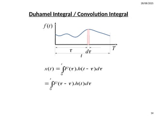
Duhamel Integral / Convolution Integral
0
0
( ) ( ). ( )
( ). ( )
t
t
x t F h t d
F h t d
  
  
 
 


( )
f t
T
 d
t

35. 28/08/2025
35
0
( )
0
0
0
0 0
( ) ( ). ( )
1
( ). sin ( ) d
sin [ ( ). cos( ) ]
cos [ ( ). cos( ) ]
A ( ) ...d ( ) ...d
Trapizoidal or simpson's rule can
n
n
n
n
n
t
t
t
d
d
t
t
d d
d
t
t
d d
d
t t
D D
x t F h t d
F e t
m
e
t F e d
m
e
t F e d
m
t B t
 

 

 
  
   

    

    

 
 


  
 


 




 
be use
to evaluate the integrals.

36. 28/08/2025
36
0 0
0 2
0
(t) cos sin ( ) ( )
1

n
t
t n
d d
n
X X
X e X t t h t f d
 
    
 

 

   
 

 
 

Complete Solution:

37. 28/08/2025
37
Estimation of ‘C’
(Half power Bandwidth method)
2
2
Energy of a signal= ( ).
1
Power ( ).
x t dt
x t dt
T
 


Dmax
max
2
D
1
r 2
r
2 2 2
max
2 2 2
1
(1 ) (2 )
2
For half power,
2 2
(1 ) (2 )
st
st st
D
r r
X
X
X X
r r





 



 

38. 28/08/2025
38
2 2 2 2
4 2 2 2
2 2 2 2
2
2 2
2
1
2
2
1 2
(1 ) (2 ) 8
, r [4 2] (1 8 ) 0
2 4 (4 2) 4(1 8 )
2
1 2 2 1
1
, 1
2
r r
or r
r
r
and r
r r
 
 
  
  
 
 

   
    
    
 
   
   
  

 
This method is only applicable to SDOF systems.

39. 28/08/2025
39
Fourier Series and transform
If, ( )
f t
Periodic function
/2
/2
/2
/2
1
/2
/2
2
( ) exp( )
1 2
x( )exp( )dt
1 2 2
( ) [ x( )exp( )dt]exp( )
Now,
2 1
; ; ;
( ) [ x(s)exp( 2 )ds]exp( 2 )
n
n
T
n T
T
T
n
n n n n n
T
T
n
i nt
x t
T
i nt
t
T T
i nt i nt
x t t
T T T
n
n f f f f
T T T
x t f i fs i ft




 

  
 


 




 




 




 
     
   


 
 
( )exp( 2 )
n
n
X f i ft f



 
 
 This is called discrete Fourier series.

40. 28/08/2025
40
0
lim ( ) ( )exp( 2 )
f
x t X f i ft df


 
 

Continuous representation…
Backward transform
1
x( ) ( )
2
Forward transform
1
( ) ( )
2
i t
i t
t X e d
X x t e dt


 




 


 





41. 28/08/2025
41
2
*
2
Energy of a signal
( ).
1
( )[ ( ) ]
2
1
X( )[ (t) ]
2
X( )[X ( )]
X( )
i t
i t
E x t dt
x t X e d dt
X e dt d
d
d


 

 

  
 


 
 


 
 

 

 






 
 


Perseval’’s Identity

42. 28/08/2025
42
Frequency Response Function
k
c
( )
x t
m
( )
f t
( )
mx cx kx f t
  
 
2
, ( ) ( ).
Putiing in the equation of motion,
1
( )
, ( ) i t
i t
and x t H
H
k m ci
Let f t e
e




 


 

0
( ) is called Frequency response function.
( ) ( ). ( ) Time Domain
X( )= ( ) ( ) Frequency Domain
t
H
x t F h t d
H F

  
  
   
 


43. 28/08/2025
43
( )
( ) ( ) ( )
1
( ) ( )
2
1
( ) ( )
2
1
( ) ( )
2
1
( ) ( )
2
1
( )
2
i
i
i t u
i t
i t
x t h t f d
h t F e d d
F h t e d d
F h u e du d
F H e d
X e d





  
   

   

 

  

 


 
 
   
 
   
 

   

 

 
 
 
   
 
 
 
 
 
 
  
 



 
 
 



44. 28/08/2025
44
Response due to Support Motion
ks
cs
ms
 
g
x t

 
x t
2
Eqn. of motion,
) )
( ) ( ) - ( )
Then,
)
( ( 0
Where, ( ) is the absolute response.
if,
( 0
,
2
g g
r g
r g r r
r r r g
r r r r r r g
t x t x t
mx c x x k x x
x t
x
m x x cx kx
or mx cx kx mx
x x x x
 




    
  
  
  
  
  
  
  

45. 28/08/2025
45
( )
0
1
( ) ( ). sin ( ) d
n
t
t
r g d
d
x t x e t
 
   

 

  


,max max
.[ ( )]
. ( , )
( , ) Spectral Displacement
s r
d
d
f k x t
k S
S


 
 
 


2
Eqn. of motion,
, c=0,
r r r g
r r n r
when
k
x x
m
mx cx kx mx
x 

 
  
  

2
( , ) . ( , )
( , ) Pseudo-Spectral Acceleration
pa n d
pa
S S
S
 

    
 



46. 28/08/2025
46
2
,max
,
. ( , ) m ( , ) m ( , )
s d n d pa
Now
f k S S S
  
      
   
Response Spectrum is the maximum response quantity of a SDOF
system for a given earthquake and damping, for the entire range of
natural frequency.
2
if,
, ,
2 .
log( ) log( ) log(2 . ) Slope of 135
log( ) log( ) log(2 . ) Slope of 45
2
i t
g
i t i t i t
r r r
pa
pv n d d
n
pv d
pa
pv
e
e i e e
S
S S f S
S f f S
S
S f f
x
x x x

  
 
 





  
   
   
   



 

47. 28/08/2025
47
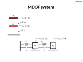
MDOF system
2 2
( ),F (t)
x t
1 1
( ),F (t)
x t
2
m
1
m
1
c 2
c
1
k 2
k
1 1
( ),F (t)
x t
2 2
( ),F (t)
x t
2
m
1
m
1 1
,
k c
2 2
,
k c

48. 28/08/2025
48
Free Body Diagram
Approach
1( )
f t
1 1
m x

1 1
c x

1 1
k x 1
m 2 1 2
( )
k x x

2 1 2
( )
c x x

 
2 ( )
f t
2 2
m x

2 2 1
( )
k x x
 2
m
2 2 1
( )
c x x

 
Dynamic equilibrium equation:
Taking summation of all forces in x direction, we get
1 1 1 1 1 1 2 1 2 2 1 2 1
2 2 2 2 1 2 2 1 2
( ) ( )
( ) ( )
( )
and,
( )
m x k x c x c x x k x x F t
m x c x x k x x F t
   
  
  
 
   
  

49. 28/08/2025
49
          
1 1 1 2 2 1 1 2 2 1 1
2 2 2 2 2 2 2 2 2
0
0
,
m x c c c x k k k x F
m x c c x k k x F
or M x C x K x F
   
             
   
       
     
 
             
  
 
 
 
Coupled Equation..

50. 28/08/2025
50
Undamped Free Vibration
Dynamic equilibrium equation:
       
   
   
       
       
2
2
2
0
,
( ) sin( ) , 1,2
( ) sin( )
( ) sin( )
Putting in the equation of motion we get,
sin( ) sin( ) 0
, sin( ) 0
For, non trivial solution,
i i
M x K x
Let
x t a t i
x t a t
x t a t
M a t K a t
or K M a t
 
 
  
    
  
 
  
  
  
    
 
  
 


   
2
0
K M

 

51. 28/08/2025
51
Numerical example
1 1
( ),F (t)
x t
2 2
( ),F (t)
x t
2
m
1
m
1 1
,
k c
2 2
,
k c
m1=10 kg
m2=15 kg
k1=100 N/m
k2=120 N/m
       
 
 
   
 
2
2
0
10 0
,
0 15
220 120
,
120 120
,
0
2.958, 27.04
1.71, 5.20
1 1
,
1.58 0.42
M x K x
Where M
and K
Now
K M
Eigen vectors a
Mode shapes



 
 
 
 

 
 

 
 
 
 
 
 

 


52. 28/08/2025
52
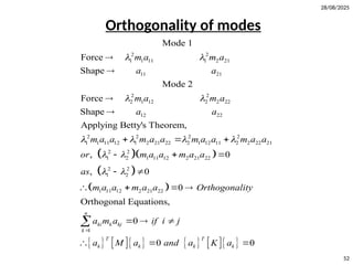
Orthogonality of modes
2 2
1 1 11 1 2 21
11 21
2
2 1
Mode 1
Force
Shape
Mode 2
Force
m a m a
a a
m a
 




  
 
2
12 2 2 22
12 22
2 2 2 2
1 1 11 12 1 2 21 22 2 1 12 11 2 2 22 21
2 2
1 2 1 11 12 2 21 22
2 2
1 2
1 11 12 2
Shape
Applying Betty's Theorem,
, 0
, 0
m a
a a
m a a m a a m a a m a a
or m a a m a a
as
m a a m

   
 
 

  
  
 
 
 
         
21 22
1
0
Orthogonal Equations,
0
0 0
n
ki k kj
k
T T
k k k k
a a Orthogonality
a m a if i j
a M a and a K a

 
  
  


53. 28/08/2025
53
Orthogonality of modes
1 1
( ),F (t)
x t
2 2
( ),F (t)
x t
2
m
1
m
1 1
,
k c
2 2
,
k c
          
     
2
2
2
( )
,
0
Applying Betty's Theorem for m and n mode
,
0
, 0
n
th th
T T
m n n m
T T
m n m n n
T
m n
T
m n
M x C x K x F t
Now
K M
K M
f f
now K M
M when m n
and K when m n
 

 
    
 
 
  
 
   


   
  
 

54. 28/08/2025
54
Damped forced vibration
          
    
             
                     
( )
Let us use the trasformation,
( )
, ( )
T T T T
M x C x K x F t
x z
M z C z K z F t
or M z C z K z F t
  
 
      
         
 
 
 
1 1
( ),F (t)
x t
2 2
( ),F (t)
x t
2
m
1
m
1 1
,
k c
2 2
,
k c

55. 28/08/2025
55
                     
      
      
     
      
( )
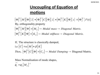
By, orthogonality property
.
.
If, The structure is classically damped,
i.e
,
T T T T
T
d
T
d
T
d
M z C z K z F t
M M Modal mass Diagonal Matrix
K K Modal stiffness Diagonal Matrix
C M K
Then C C Modal D
 
         
    
    
 
   
 
 
1
Diagonal Matrix.
Mass Normalisation of mode shapes,
n n d
amping
M
 




Uncoupling of Equation of
motions

56. 28/08/2025
56
Damped forced vibration
          
    
             
                     
   
      
    
    
2
( )
Let us use the trasformation,
( )
, ( )
, is mass normalised mode shapes, and is classical damping,
then,
, 2
T T T T
T
T
n
T
M x C x K x F t
x z
M z C z K z F t
or M z C z K z F t
if C
M I
K
and C



  
 
      
         

  
 
   
  
 
 
 
 
n n
 
1 1
( ),F (t)
x t
2 2
( ),F (t)
x t
2
m
1
m
1 1
,
k c
2 2
,
k c

57. 28/08/2025
57
Solution of α and β
     
              
 
    2
2
1 1 1
2
2 2 2
Let,
, normalised mode shapes
2
, First two modes,
2
2
, Two equations, and two unknowns are present,
exact solution
T T T
n n n
C M K
C M K
if Mass
I
Consideri ng
When
 
 
    

   
   
 
 
        
 
 
    
 
 
can be found.
, More than two equations, and two unknowns are present,
Least square solution can be found.
When

58. 28/08/2025
58
Damped vibration under
support motion
           
 
    
              
                      
        
    
    
  
2
(t)
1
.. influence vector
1
Let us use the trasformation,
(t)
, (t)
2 (t)
2
g
g
T T T T
g
T
n n n g
T
n
M x C x K x M r x
r
x z
M z C z K z M r x
or M z C z K z M r x
M r
I z z z x
M
I z
  
 
 
  
 
 
 
 
 
 
 
      
         

 
  
 
 
 
  

 

 

 
      
    
    
2
( )
, ( )
n n d
d
T
T
z z F t
where F t Modal Force
M r
Modal Mass Participation Factor
M

 
 
 
 



 

1( )
x t
2 ( )
x t
2
m
1
m
1 1
,
k c
2 2
,
k c
( )
g
x t


59. 28/08/2025
59
Time domain solution
        
    
    
    
 
2
0 0
0 0
0 0
0
2 ( )
Initial conditions,
,
Using complete time domain solution for SDOF systems,
z (t) cos sin ( ) ( )
i ni
n n n d
t t
t
t
i i d i d ni dni
I z z z F t
X Z
X Z
and X Z
e A t B t h t F d
 
  
    
 
 

 
  
 
 
  
 
   

 
 

60. 28/08/2025
60
Frequency domain solution
        
   
 
2
2
(t)
Using fourier transform,
1
x( ) x( )
2
1 1
x( ) x( )
2 2
1 1
x( ) ( )
2 2
, {[K M ] ( ) F( )}
i t
i t i t
i t i t
i t
M x C x K x F
t e d
M e d C i e d
K e d F e d
or i C X e

 
 

 

     
 
   
 
   

 
 
   
 
   
  

   
  
   
   
   
 
   
   
  

 
 
 
2
2 1
2 1
0
The dynamic equilibrium holds for every ,
so using localisation theorem
[K M ] ( ) F( ) 0
, ( ) [K M ] F( )
( ) ( ) F( )
( ) [K M ]
d
i C X
or X i C
X H
H i C


   
   
  
  

 



   
  
 
  


61. 28/08/2025
61
Frequency domain solution in
modal coordinates
        
  
2
2
2 2
2 2
2 ( )
r equation will be
2 ( )
1
( ) ( ) ( )
2
( ) ( ) ( )
1
( )
2
Now,
( ) ( )
n n n d
th
r
r r r r r r d
r
r d
r r r
r
r r d
r
r r r
I z z z F t
z z z F t
z F
i
z H F
H
i
X Z
  
  
 
   
  

   
 
 
 
  
 
  
 
 
 
 
 
 
 
 