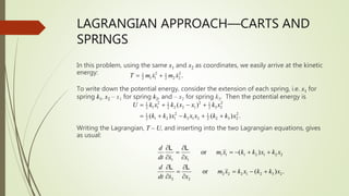
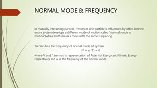
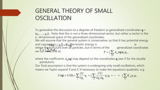
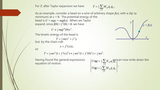
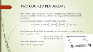
This document summarizes classical dynamics and small amplitude oscillations. It discusses oscillatory motion near equilibrium positions and developing the theory using Lagrange's equations. Normal modes of coupled oscillating systems are explored, where the normal coordinates represent eigenvectors that oscillate at characteristic frequencies. The principles of superposition and matrix representations are used to analyze examples like two coupled pendulums and a system of two masses connected by three springs.

1. CLASSICAL DYNAMICS
SMALL AMPLITUDE OSCILLATION
NAME : HARSH SHARMA
ROLL NO. : 31830219
UNIVERSITY ROLL NO. : 18036567036
COURSE : BSC PHYSICS(HONS.)

2. SMALL OSCILLATION
 Any mechanical system can perform oscillations in the neighbourhood of a position of
stable equilibrium. These oscillations are an extremely important feature of the system
whether they are intended to occur (as in a pendulum clock), or whether they are
undesirable (as in a suspension bridge!). Analogous oscillations occur in continuum
mechanics and in quantum mechanics. Here we present the theory of such oscillations
for conservative systems under the assumption that the amplitude of the oscillations is
small enough so that the linear approximation is adequate.
 The best way to develop the theory of small oscillations is to use Lagrange's equations.
We will show that it is possible to approximate the expressions for T and V from the
start so that the linearized equations of motion are obtained immediately. The theory is
presented in an elegant matrix form which enables us to make use of concepts from
linear algebra, such as eigenvalues and eigenvectors.

3. EQUILIBRIUM CONDITION
Let a particle of mass ‘m’ moving under the potential 𝑉 𝑥 = 𝑉0 + 1/2𝑘𝑥2
,has the
frequency of oscillation 𝑤 = 𝑘/𝑚 about stable equilibrium point. Then we can expand
𝑉 𝑥 about 𝑥0 using Taylor Series Expansion.
𝑉 𝑥 = 𝑉0 +
𝑥−𝑥𝑜
1!
𝑑𝑣
𝑑𝑥
|𝑥 = 𝑥𝑜 +
𝑥−𝑥𝑜
2
2!
𝑑2𝑣
𝑑𝑥2 |𝑥 = 𝑥𝑜+ …
In the above expression (𝑥 − 𝑥𝑜) is displacement from stable equilibrium point.
At Stable Equilibrium,
𝑑𝑣
𝑑𝑥
|𝑥 = 𝑥𝑜 = 0
Since (𝑥 − 𝑥𝑜) is small therefore higher term can be neglected ,
𝑉 𝑥 = 𝑉0 + 1/2 x − xo
2
𝑑2
𝑣
𝑑𝑥2
|𝑥 = 𝑥𝑜
and Force 𝐹 = −
𝑑𝑣
𝑑𝑥
= −
2 𝑥−𝑥𝑜
2
𝑑2𝑣
𝑑𝑥2 |𝑥 = 𝑥𝑜
𝐹 = −𝑘(𝑥 − 𝑥𝑜) in case of SHM

4. STABLE EQUILIBRIUM
 The slope of Potential Energy curve(Force) is zero.
 𝐹 = −
𝑑𝑣
𝑑𝑥
= 0

𝑑2𝑣
𝑑𝑥2 =+ve
 Potential Energy is minimum at this point.
 Small displacement from this point results small bounded motion about the point
of equilibrium.
 Ex: Bar pendulum at rest

5. UNSTABLE EQUILIBRIUM
 The slope of Potential Energy curve(Force) is zero.
 𝐹 = −
𝑑𝑣
𝑑𝑥
= 0

𝑑2𝑣
𝑑𝑥2 =-ve
 Potential Energy is maximum at this point.
 Small displacement from this point results small unbounded motion about the
point of equilibrium.
 Ex: Rod standing on its one end, egg is made to stand on one end

6. NEUTRAL EQUILIBRIUM
 The slope of Potential Energy curve(Force) is zero.
 𝐹 = −
𝑑𝑣
𝑑𝑥
= 0

𝑑2𝑣
𝑑𝑥2 = 0
 Potential Energy is constant at this point.
 Small displacement from this point results no change about the point of
equilibrium.

8. NORMAL MODE & FREQUENCY
In mutually interacting particle, motion of one particle is influenced by other and the
entire system develops a different mode of motion called “normal mode of
motion”(where both masses move with the same frequency).
To calculate the frequency of normal mode of system
𝑉 − 𝑤2
𝑇 = 0
where V and T are matrix representation of Potential Energy and Kinetic Energy
respectively and w is the frequency of the normal mode.

9. KINETIC AND POTENTIAL ENERGY IN
NORMAL COORDINATES
Kinetic Energy : 𝑇 =
1
2
𝑚𝑥1
2
+
1
2
𝑚𝑥2
2
=
1
2
𝑚 𝑋1 + 𝑋2
2
+
1
2
𝑚 𝑋1 − 𝑋2
2
=
1
2
𝑚𝑋1
2
+
1
2
𝑚𝑋2
2
Potential Energy : 𝑉 =
1
2
𝑘𝑥1
2
=
1
2
𝑘𝑥2
2
+
1
2
𝑘′
𝑥1 − 𝑥2
2
=
1
2
𝑘 𝑋1 + 𝑋2
2
+ 𝑋1 − 𝑋2
2
+
1
2
𝑘′
2𝑋2
2
= 𝑘 𝑋1
2
+ 𝑋2
2
+ 2𝑘′𝑋2
2
Lagrangian : 𝐿 =
1
2
𝑚 𝑋1
2
+ 𝑋2
2
− 𝑘 𝑋1
2
+ 𝑋2
2
− 2𝑘′
𝑋2
2
Both T and V are homogenous quadratic functions.

10. GENERAL THEORY OF SMALL
OSCILLATION
To generalize the discussion to n degrees of freedom (n generalized coordinates q =
(q1, …, qn)). Note that this is not a three-dimensional vector, but rather a vector in the
n -dimensional space of the generalized coordinates.
We will assume that the general system is conservative, so that it has potential energy
and Lagrangian L = T – U. The kinetic energy is w
where the sum runs over all particles, but in terms of the generalized coordinates
we can write this as
where the coefficients Ajk(q) may depend on the coordinates q (see T for the double
pendulum).
Our final assumption is that the system is undergoing only small oscillations, which
means we Taylor expand T and U if necessary to make the equations quadratic, e.g.
1
( ,..., ) ( )
n
U q q U
 q
2
1
2 ,
T m 
  r 1
2
,
( ) ,
jk j k
j k
T A q q
  q
2
1 1
2 2
, ,
( ) (0) .
j j k jk j k
j j k j k
j j k
U U
U U q q q K q q
q q q
 
    
  
  
q

11. For T, after Taylor expansion we have
As an example, consider a bead on a wire of arbitrary shape f(x), with a dip (a
minimum) at x = 0. The potential energy of the
bead is U = mgy = mgf(x). When we Taylor
expand, since f(0) = f (0) = 0, we have
The kinetic energy of the bead is
but, by the chain rule
so
Having found the general expressions we can now write down the
equation of motion.
1
2
,
,
jk j k
j k
T M q q
 
y = f(x)
x
y
2
1
2 (0) .
U mgf x


2 2
1
2 ( ),
T m x y
 
( ) ,
y f x x


2 2 2 2 2
1 1 1
2 2 2
(1 ( ) ) (1 (0) ) .
T mx f x mx f mx
 
    
1
2
,
1
2
,
( )
,
( )
jk j k
j k
jk j k
j k
U K q q
T M q q
 

 
 

 
 


q
q

12. TWO COUPLED PENDULUMS
We’ll take two equal pendulums, coupled by a light spring. We take the spring
restoring force to be directly proportional to the angular difference between the
pendulums.
For small angles of oscillation, we take the Lagrangian to be
𝐿 =
1
2
𝑚𝑙2𝜃
2
1
+
1
2
𝑚𝑙2𝜃
2
2
−
1
2
𝑚𝑙2𝜃
2
1
−
1
2
𝑚𝑙2𝜃
2
2
−
1
2
𝐶(𝜃1 − 𝜃2)
Denoting the single pendulum frequency by 𝑤𝑜, the equations of motion are (𝑤𝑜
2
=
𝑔
𝑙
, 𝑘 =
𝐶
𝑚𝑙2 , 𝑠𝑜 𝑘 = 𝑇−2)
𝜃1 = −𝑤𝑜
2𝜃1 − 𝑘(𝜃1 − 𝜃2)
𝜃2 = −𝑤𝑜
2
𝜃2 − 𝑘(𝜃2 − 𝜃1)
We look for a periodic solution,
𝜃1 𝑡 = 𝐴1𝑒𝑖𝑤𝑡 𝜃2 𝑡 = 𝐴2𝑒𝑖𝑤𝑡

13. The equations become (in matrix notation):
𝑤2 𝐴1
𝐴2
=
𝑤𝑜
2
+ 𝑘 −𝑘
−𝑘 𝑤𝑜
2 + 𝑘
𝐴1
𝐴2
Denoting the 2×2 matrix by M,
𝑀𝐴 = 𝑤2
𝐴, 𝐴 =
𝐴1
𝐴2
This is an eigenvector equation, with 𝑤2
the eigenvalue, found by the standard
procedure:
∆ 𝑀 − 𝑤2
𝐼 = ∆
𝑤𝑜
2
+ 𝑘 −𝑘
−𝑘 𝑤𝑜
2
+ 𝑘
= 0
Solving, 𝑤2
= 𝑤𝑜
2
+ 𝑘 ± 𝑘, that is,
𝑤2
= 𝑤𝑜
2
, 𝑤2
= +2𝑘
The corresponding eigenvectors are (1,1) and (1,−1).

14. NORMAL MODES
The physical motion corresponding to the amplitudes eigenvector (1,1) has two
constants of integration (amplitude and phase), often written in terms of a single
complex number, that is,
𝜃1(𝑡)
𝜃2(𝑡)
=
1
1
𝑅𝑒 𝐵𝑒𝑖𝑤𝑜𝑡 =
𝐴𝑐𝑜𝑠 𝑤𝑜𝑡 + 𝛿
𝐴𝑐𝑜𝑠 𝑤𝑜𝑡 + 𝛿
, 𝐵 = 𝐴𝑒𝑖𝛿
with A,δ real.
Clearly, this is the mode in which the two pendulums are in sync, oscillating at their
natural frequency, with the spring playing no role.
In physics, this mathematical eigenstate of the matrix is called a normal mode of
oscillation. In a normal mode, all parts of the system oscillate at a single frequency,
given by the eigenvalue.

15. The other normal mode,
𝜃1(𝑡)
𝜃2(𝑡)
=
1
−1
𝑅𝑒 𝐵𝑒𝑖𝑤0𝑡
=
𝐴𝑐𝑜𝑠 𝑤′𝑡 + 𝛿
−𝐴𝑐𝑜𝑠 𝑤′𝑡 + 𝛿
, 𝐵 = 𝐴𝑒𝑖𝛿
where we have written 𝑤′ = 𝑤𝑜
2
+ 2𝑘. Here the system is oscillating with the single
frequency 𝑤′
, the pendulums are now exactly out of phase, so when they part the
spring pulls them back to the center, thereby increasing the system oscillation
frequency.
The matrix structure can be clarified by separating out the spring contribution:
𝑀 =
𝑤𝑜
2 + 𝑘 −𝑘
−𝑘 𝑤𝑜
2 + 𝑘
= 𝑤𝑜
2 1 0
0 1
+ 𝑘(
1 −1
−1 1
)
All vectors are eigenvectors of the identity, of course, so the first matrix just
contributes 𝑤𝑜
2 to the eigenvalue. The second matrix is easily found to have
eigenvalues are 0,2, and eigenstates (1,1) and (1,−1).

16. PRINCIPLE OF SUPERPOSITION
The equations of motion are linear equations, meaning that if you multiply a solution by a
constant, that’s still a solution, and if you have two different solutions to the equation, the
sum of the two is also a solution. This is called the principle of superposition.
The general motion of the system is therefore
𝜃1 = 𝐴𝑒𝑖𝑤0𝑡
+ 𝐵𝑒
𝑖
𝑤𝑜
2
+ 2𝑘𝑡
𝜃2 = 𝐴𝑒𝑖𝑤0𝑡
− 𝐵𝑒
𝑖
𝑤𝑜
2
+ 2𝑘𝑡
where it is understood that A,B are complex numbers and the physical motion is the real
part.
This is a four-parameter solution: the initial positions and velocities can be set arbitrarily,
completely determining the motion.

17. GENERAL PROBLEM OF COUPLED
OSCILLATIONS
The results of our study of the coupled harmonic oscillator problem results in a
number of different observations:
• The coupling in a system with two degrees of freedom results in two characteristic
frequencies.
• The two characteristic frequencies in a system with two degree of freedom are
pushed towards lower and higher energies compared to the non-coupled
frequency.

18. LONGITUDINAL OSCILLATION (TWO
MASSES AND THREE SPRINGS)
Consider the situation shown in the figure at right. There are two cars of masses m1
and m2, and three springs of spring constants k1, k2 and k3, and we want to obtain the
equations of motion for the two cars.
Let’s use the Newtonian approach. The equilibrium positions of the two cars are
shown by the lines, and we will use coordinates x1 and x2 relative to those.
The forces on m1 are k1x1 to the left, and k2(x2 -x1) to the right, so its equation of
motion is Likewise:
1 1 1 1 2 2 1
1 2 1 2 2
( )
( ) ,
m x k x k x x
k k x k x
 -  -
 -  
2 2 2 1 2 3 2
( ) .
m x k x k k x
 - 

19. The two coupled equations of motion:
can be written more compactly using matrix notation, as where
Notice that this is a generalization of the single oscillator, which you can see by setting
k2 and k3 = 0. Note also that if the coupling spring, k2 = 0, then the two equations
become uncoupled and describe two separate oscillators.
We will find complex solutions z(t) = aeiwt, but you can imagine that we might have
more than one frequency of oscillation, since we have two ms and 3 ks. It
turns out that we only need to assume one frequency initially, but we will arrive at an
equation for w that is satisfied by more than one frequency.
Let’s try the solutions:
1 1 1 2 1 2 2
2 2 2 1 2 3 2
( )
( ) ,
m x k k x k x
m x k x k k x
 -  
 - 
1 2 2
1 1
2 2 3
2 2
0
, , and .
0
k k k
x m
k k k
x m
 -
 
   
    
    - 
     
x M K
,
 -
Mx Kx
1
2
1 1 1 1
2 2 2 2
( )
( ) , where .
( )
i
i t i t
i
z t a a e
t e e
z t a a e

w w



-
-
 
     
      
     
       
z a a
/ ,
k m
w 

20. When we write the solution in terms of complex exponentials, we will ultimately have
to keep only the real part of the solution, i.e. x(t) = Re z(t).
When we substitute z(t) into we find the relation
so the following equation must be satisfied:
Clearly, if we ignore the trivial solution a = 0 (no motion at all), we must have
Since these are two x two matrices, you can see that the determinant will give a
quadratic equation for w2, with two solutions (two roots).
This implies that there are two frequencies at which our system will oscillate, and these
are called normal modes of the system. We could find them for this system with two
different masses and three different spring constants, but it is complicated and not
very interesting. Let’s look at simpler systems.
,
 -
Mx Kx
2
,
i t i t
e e
w w
w
-  -
Ma Ka
2
( ) 0.
w
- 
K M a
2
det( ) 0.
w
- 
K M

21. IDENTICAL SPRINGS AND EQUAL MASSES
For this case, the matrices M and K become:
We then need to find the determinant of
which is
Setting this to zero, we find two solutions (the two normal mode frequencies):
Now that we have the frequencies, we must still solve the equation
We do this twice, once for each frequency, to obtain the motion x(t) for the two oscillating carts.
0 2
, and .
0 2
m k k
m k k
-
   
 
   
-
   
M K
2
2
2
2
,
2
k m k
k k m
w
w
w
 
- -
-   
- -
 
K M
2 2 2 2 2 2
det( ) (2 ) ( )(3 ),
k m k k m k m
w w w w
-  - -  - -
K M
1 2
3
, and .
k k
m m
w w w w
   
2
( ) 0.
w
- 
K M a

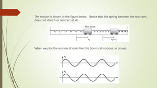
22. FIRST NORMAL MODE
First insert , so that the relation
As a check, you can see that the determinant of this matrix is zero. The solutions are
then
These are both the same equation, and simply says that a1 = a2 = Ae-i. Since
we finally have
That is, both carts move in unison:
2
1 .
k k
k k
w
-
 
-   
-
 
K M
1 /
k m
w 
1 1 2
2
2 1 2
0
1 1
( ) 0 or .
0
1 1
a a a
k
a a a
w
- 
-  
 
-  
 
  -  
-
   
K M a
1 1
1 1 ( )
2 2
( )
( ) ,
( )
i t i t
z t a A
t e e
z t a A
w w 
-
     
  
     
 
   
z
1
1
2
( )
( ) cos( ).
( )
x t A
t t
x t A
w 
   
  -
   
 
 
x
1 1
2 1
( ) cos( )
[first normal mode].
( ) cos( )
x t A t
x t A t
w 
w 
 -
 -

23. The motion is shown in the figure below. Notice that the spring between the two carts
does not stretch or contract at all.
When we plot the motion, it looks like this (identical motions, in phase).

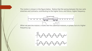
24. SECOND NORMAL MODE
Now insert , so that the relation
As a check, you can see that the determinant of this matrix is zero. The solutions are then
These are again both the same equation, and simply says that a1 = -a2 = Ae-i. Since
we finally have
That is, both carts move oppositely:
2
1 .
k k
k k
w
- -
 
-   
- -
 
K M
2 3 /
k m
w 
1 1 2
2
2 1 2
0
1 1
( ) 0 or .
0
1 1
a a a
k
a a a
w
 
 
 
-  - 
 
   
   
K M a
2 2
1 1 ( )
2 2
( )
( ) ,
( )
i t i t
z t a A
t e e
z t a A
w w 
-
     
  
     
-
 
   
z
1
2
2
( )
( ) cos( ).
( )
x t A
t t
x t A
w 
   
  -
   
-
 
 
x
1 2 nd
2 2
( ) cos( )
[2 normal mode].
( ) cos( )
x t A t
x t A t
w 
w 
 -
 - -

25. The motion is shown in the figure below. Notice that the spring between the two carts
stretches and contracts, contributing to the higher force, and hence, higher frequency.
When we plot the motion, it looks like this (identical motions, in phase, but at a higher
frequency w2).

26. GENERAL MOTION
Although these are the only two normal modes for the oscillation, the general
oscillation is a combination of these two modes, with possibly different amplitudes
and phases depending on initial conditions.
The resulting motion is surprisingly complicated, but deterministic. Because
is an irrational ratio, the motion never repeats itself, except in the case that either A1 or
A2 = 0.
1 1 1 2 2 2
1 1
( ) cos( ) cos( ).
1 1
t A t A t
w  w 
   
 -  -
   
-
   
x
2 1
3
w w

Motion for
A1 = 1, 1 = 0
A2 = 0.7, 2 = p/2

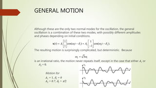
27. NORMAL COORDINATES
If the motion seems complicated, you should realize that there is an underlying
simplicity that is masked by our choice of coordinates. We can just as easily choose
for our coordinates the so-called normal coordinates
Using these coordinates, as you can easily check, the two normal modes are no longer
mixed, but instead we have:
1
1 1 2
2
1
2 1 2
2
( )
( ).
x x
x x


 
 -
1 1
2
1
2 2
( ) cos( )
. [first normal mode]
( ) 0
( ) 0
. [second normal mode]
( ) cos( )
t A t
t
t
t A t
 w 


 w 
 - 

 
 

 - 

28. LAGRANGIAN APPROACH—CARTS AND
SPRINGS
In this problem, using the same x1 and x2 as coordinates, we easily arrive at the kinetic
energy:
To write down the potential energy, consider the extension of each spring, i.e. x1 for
spring k1, x2 – x1 for spring k2, and – x2 for spring k3. Then the potential energy is
Writing the Lagrangian, T – U, and inserting into the two Lagrangian equations, gives
as usual:
2 2
1 1
1 1 2 2
2 2 .
T m x m x
 
2 2 2
1 1 1
1 1 2 2 1 3 2
2 2 2
2 2
1 1
1 2 1 2 1 2 2 3 2
2 2
( )
( ) ( ) .
U k x k x x k x
k k x k x x k k x
  - 
  -  
1 1 1 2 1 2 2
1 1
2 2 2 1 2 3 2
2 2
or ( )
or ( ) .
d
m x k k x k x
dt x x
d
m x k x k k x
dt x x
 
  -  
 
 
  - 
 
L L
L L

29. REFERENCES
 Classical Mechanics, By JC Upadhyaya
 https://galileoandeinstein.phys.virginia.edu/
 http://electron6.phys.utk.edu/
 https://www2.physics.ox.ac.uk/
 Wikipedia and various articles