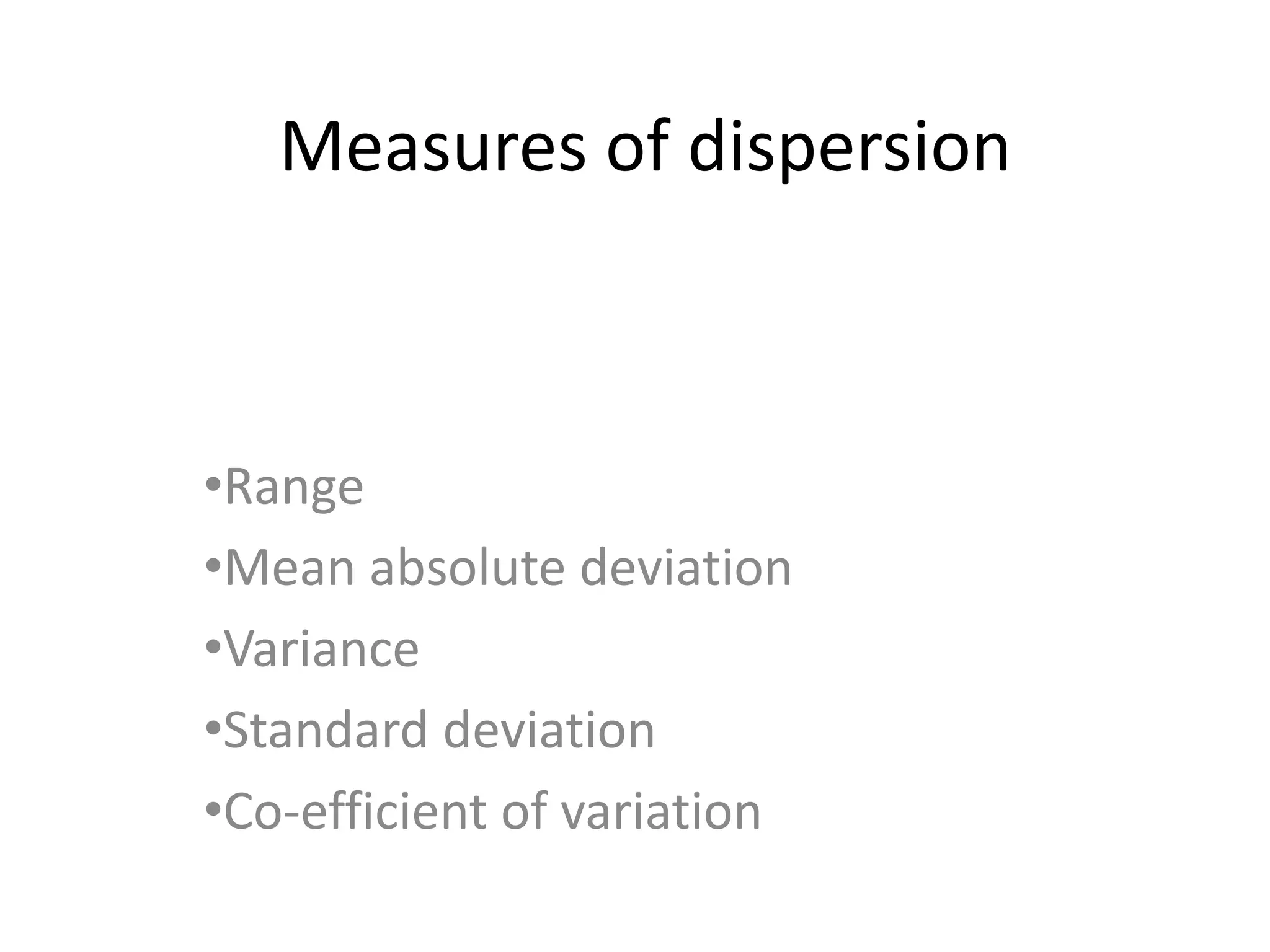
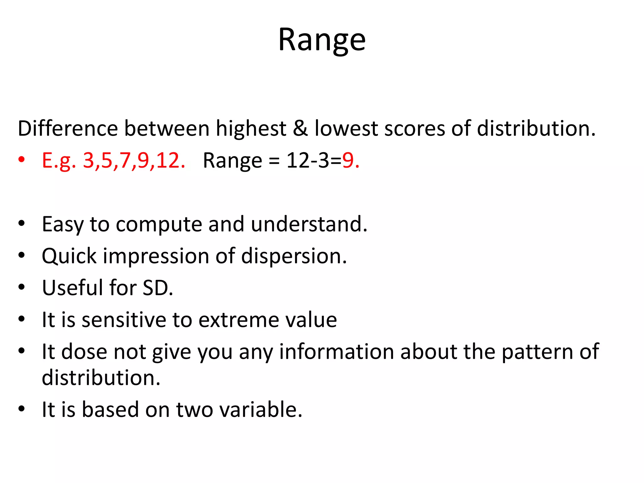
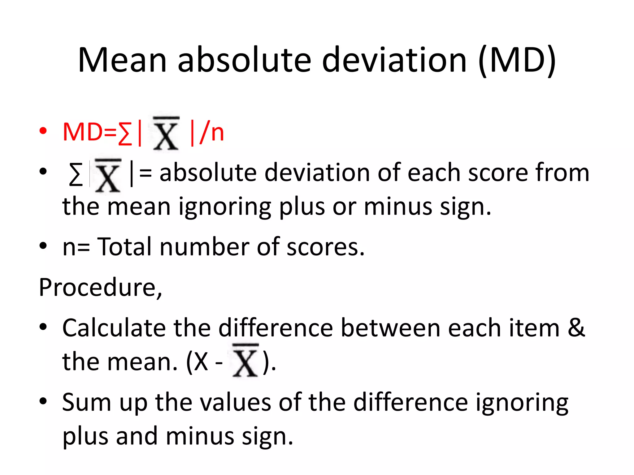
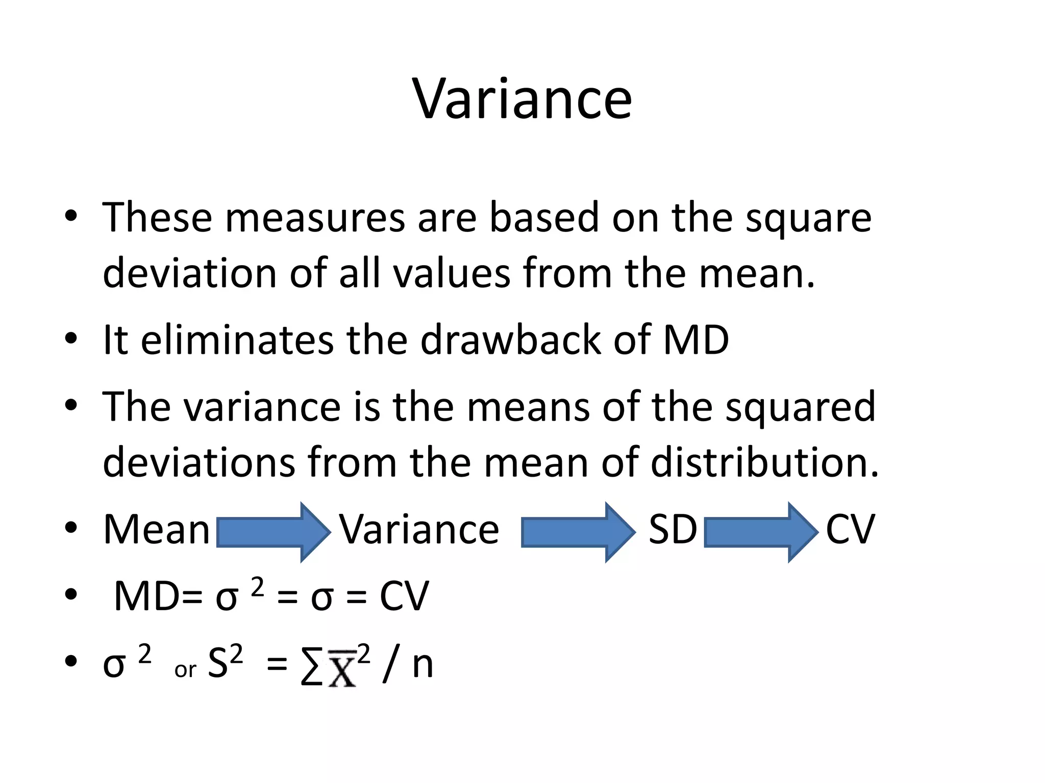
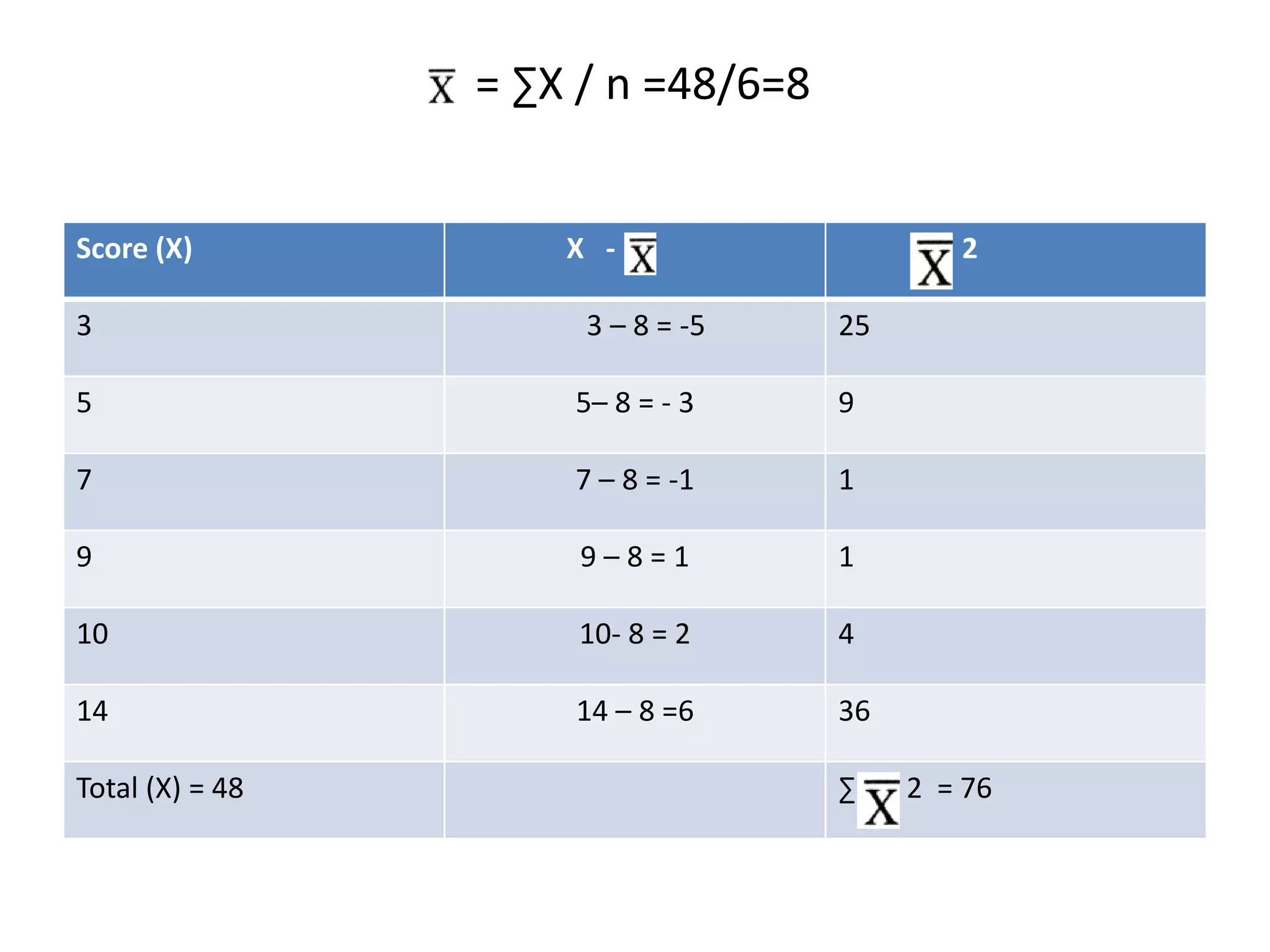
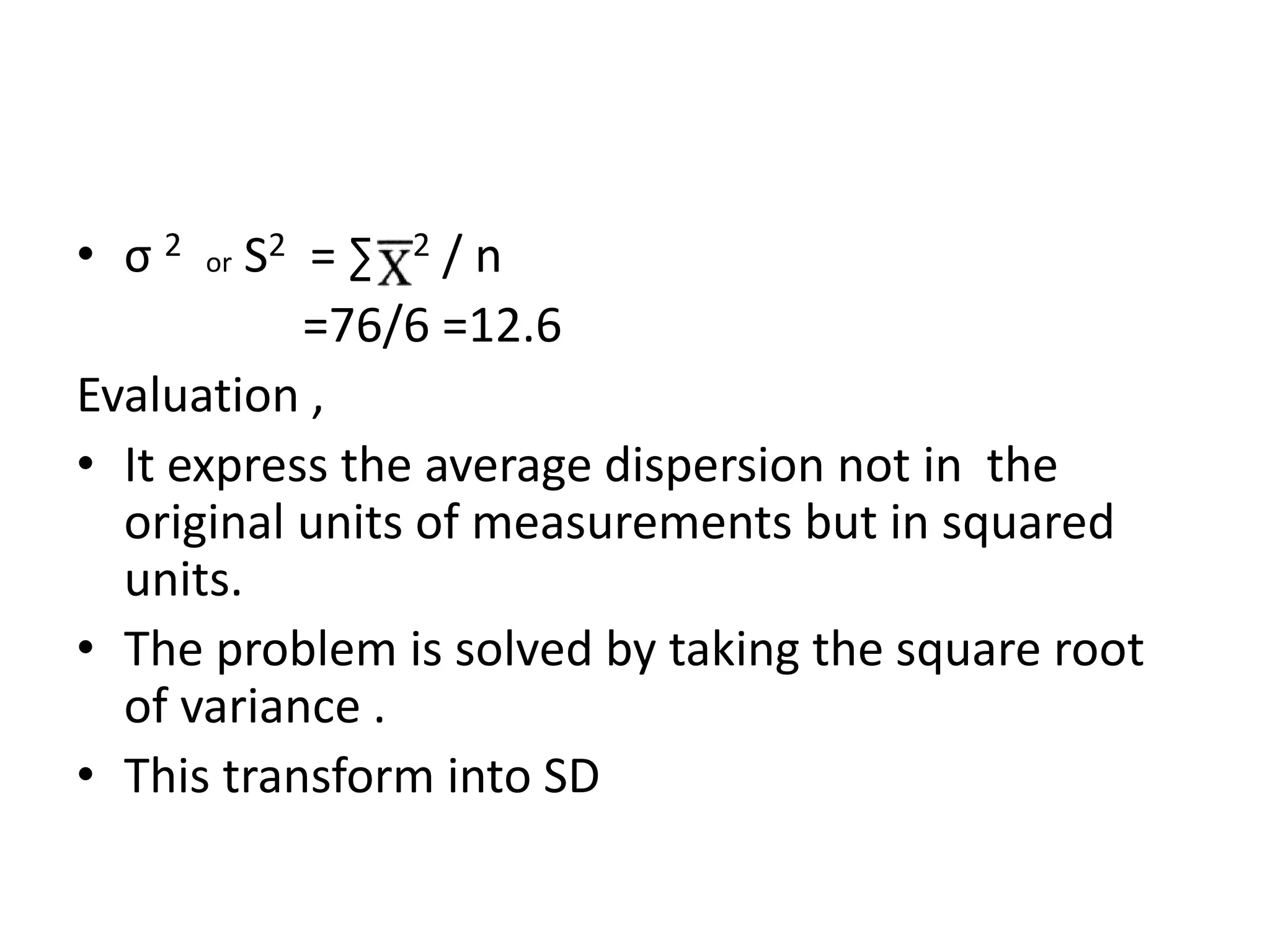
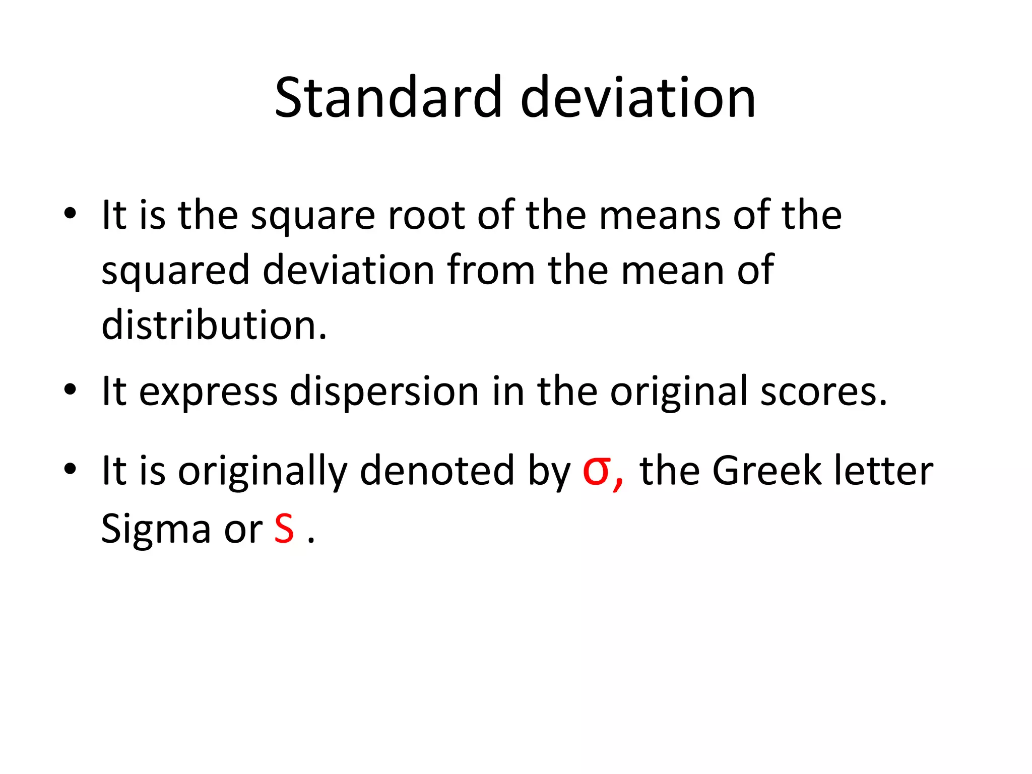
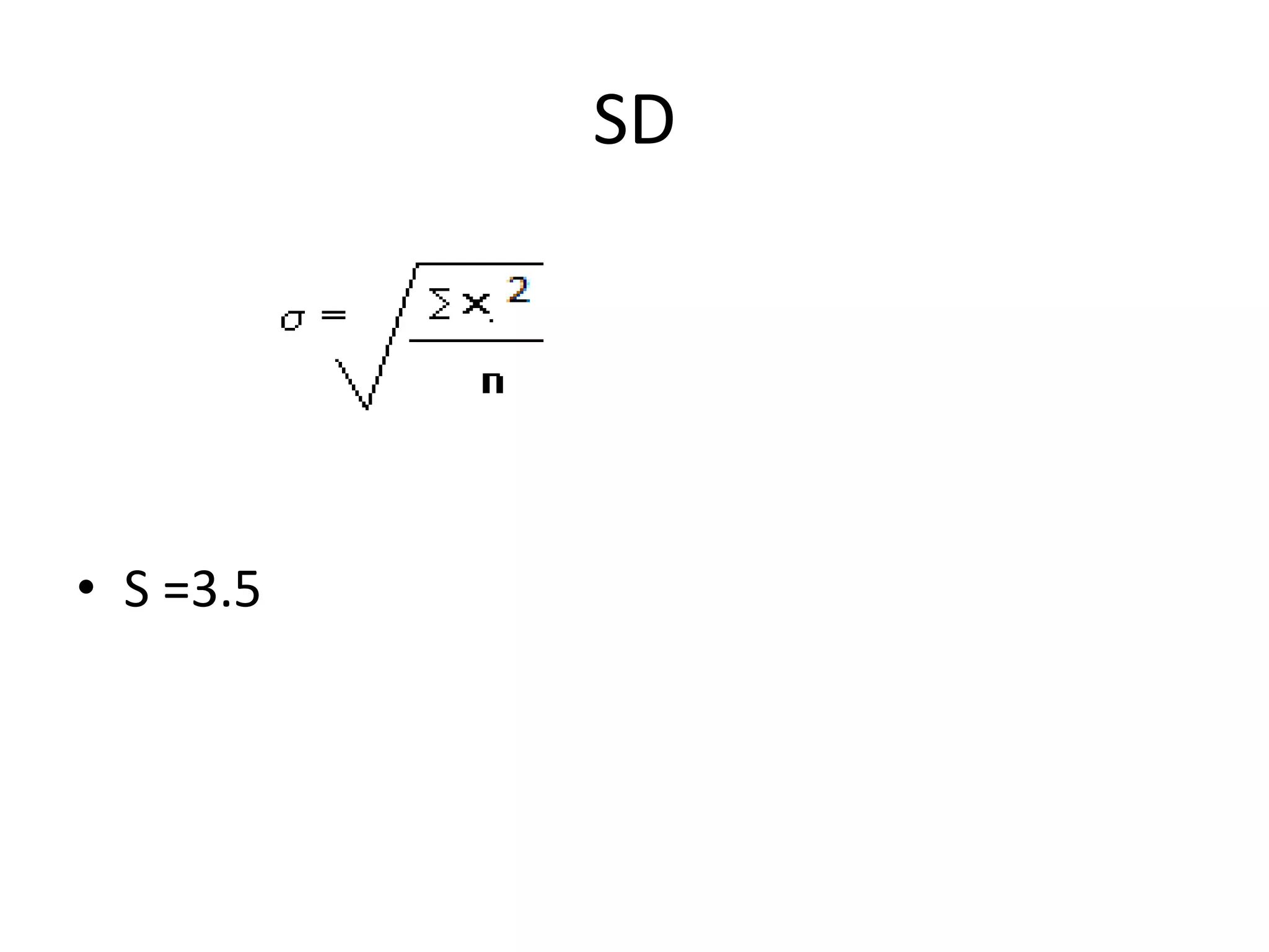
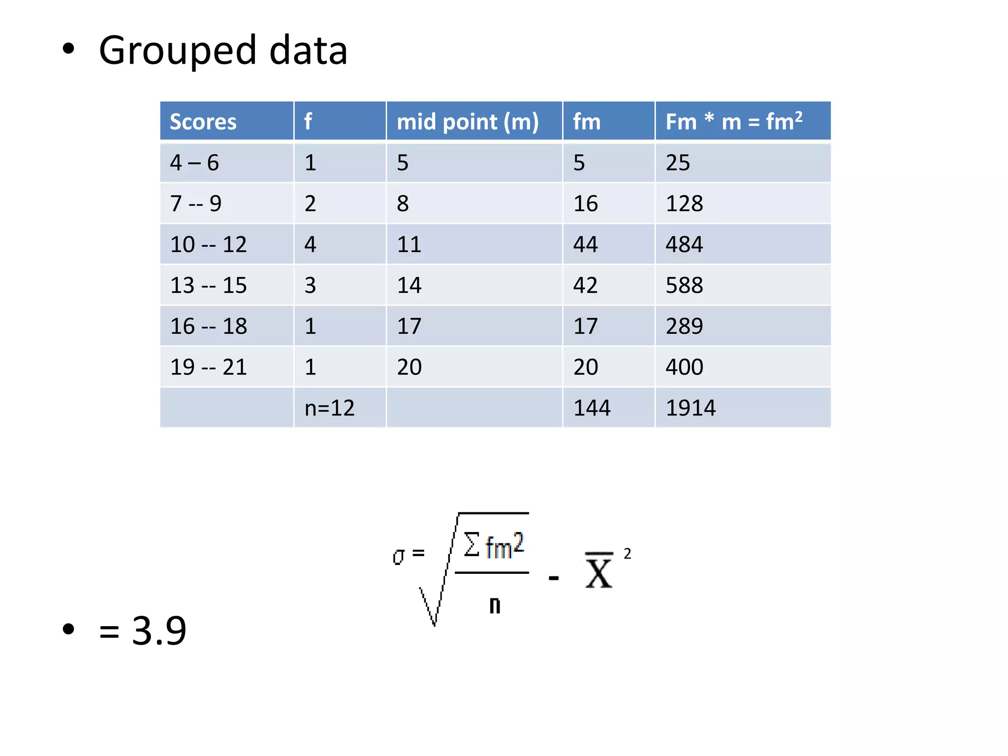
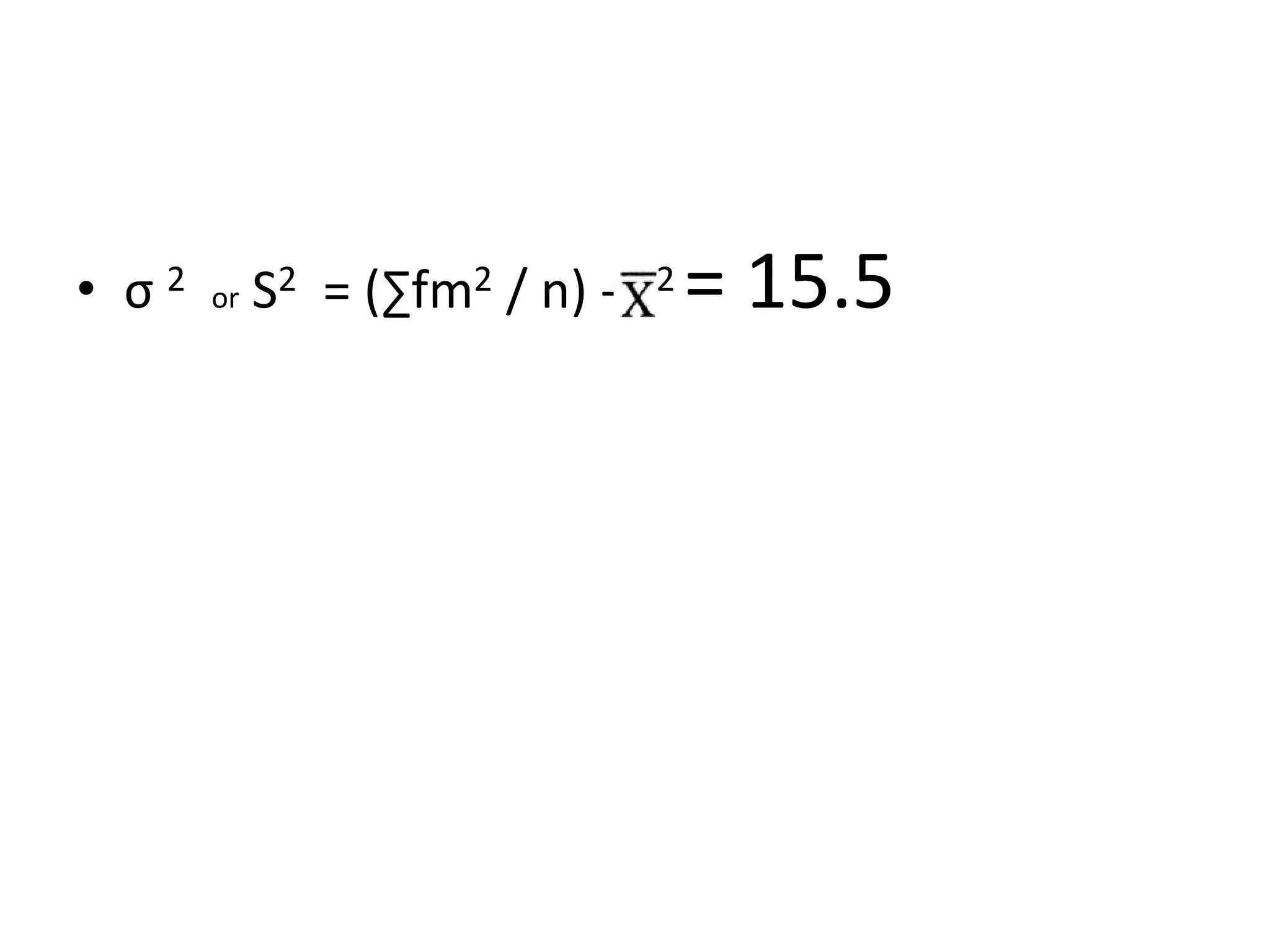
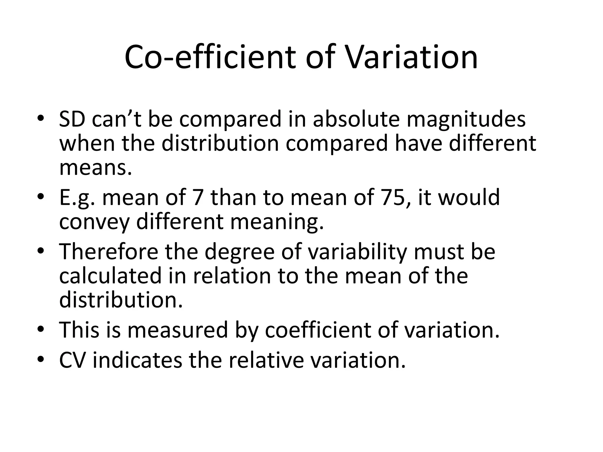
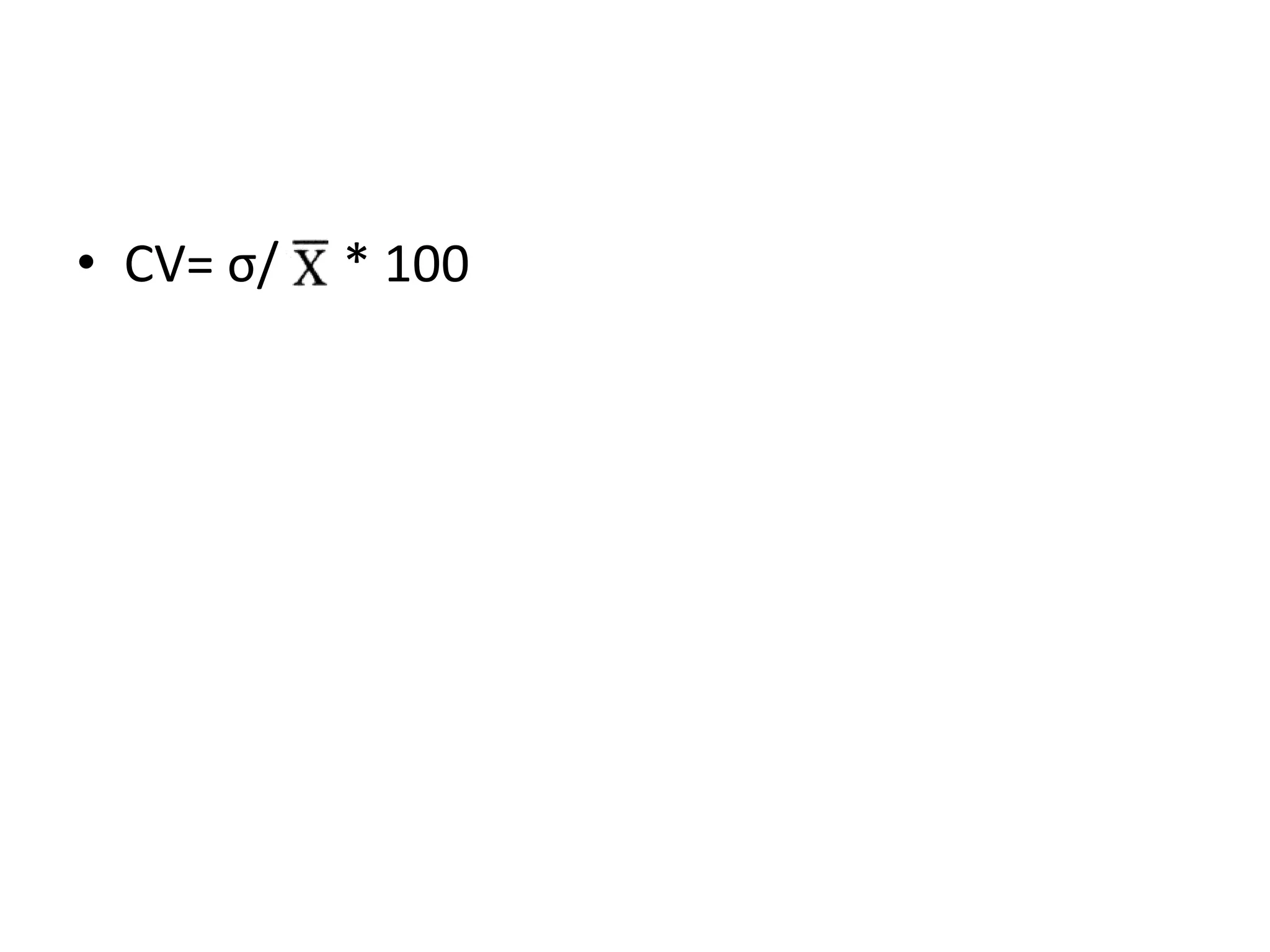
This document defines and explains several common measures of dispersion used in statistics including range, mean absolute deviation, variance, standard deviation, and coefficient of variation. Range is the difference between the highest and lowest values. Mean absolute deviation measures the average distance between values and the mean. Variance and standard deviation both measure how spread out numbers are by taking the average of the squared distances from the mean, with standard deviation being the square root of variance. Coefficient of variation expresses standard deviation as a percentage of the mean to allow comparison between data sets with different means.

1. Measures of dispersion
•Range
•Mean absolute deviation
•Variance
•Standard deviation
•Co-efficient of variation

2. Range
Difference between highest & lowest scores of distribution.
• E.g. 3,5,7,9,12. Range = 12-3=9.
• Easy to compute and understand.
• Quick impression of dispersion.
• Useful for SD.
• It is sensitive to extreme value
• It dose not give you any information about the pattern of
distribution.
• It is based on two variable.

3. Mean absolute deviation (MD)
• MD=∑│ │/n
• ∑│ │ │= absolute deviation of each score from
the mean ignoring plus or minus sign.
• n= Total number of scores.
Procedure,
• Calculate the difference between each item &
the mean. (X - ).
• Sum up the values of the difference ignoring
plus and minus sign.

4. = 40/5=8
Score (X) X -
4 4 – 8 = -4 4
6 6 – 8 = - 2 2
8 8 – 8 = 0 0
10 10 – 8 = 2 2
12 12- 8 = 4 4
Total (X) = 40 ∑ = 12

5. • MD= 12/5 = 2.4
• Evaluation –
• It represents the overall dispersion.
• MD value is not amenable to mathematical
manipulations.
• Hence MD is not useful for advance statistical
analysis.

6. Variance
• These measures are based on the square
deviation of all values from the mean.
• It eliminates the drawback of MD
• The variance is the means of the squared
deviations from the mean of distribution.
• Mean Variance SD CV
• MD= σ 2 = σ = CV
• σ 2 or S2 = ∑ 2 / n

7. = ∑X / n =48/6=8
Score (X) X - 2
3 3 – 8 = -5 25
5 5– 8 = - 3 9
7 7 – 8 = -1 1
9 9 – 8 = 1 1
10 10- 8 = 2 4
14 14 – 8 =6 36
Total (X) = 48 ∑ 2 = 76

8. • σ 2 or S2 = ∑ 2 / n
=76/6 =12.6
Evaluation ,
• It express the average dispersion not in the
original units of measurements but in squared
units.
• The problem is solved by taking the square root
of variance .
• This transform into SD

9. Standard deviation
• It is the square root of the means of the
squared deviation from the mean of
distribution.
• It express dispersion in the original scores.
• It is originally denoted by σ, the Greek letter
Sigma or S .

10. SD
• S =3.5

11. • Grouped data
• = 3.9
Scores f mid point (m) fm Fm * m = fm2
4 – 6 1 5 5 25
7 -- 9 2 8 16 128
10 -- 12 4 11 44 484
13 -- 15 3 14 42 588
16 -- 18 1 17 17 289
19 -- 21 1 20 20 400
n=12 144 1914
2
-

12. • σ 2 or S2 = (∑fm2 / n) - 2 = 15.5

13. Evaluation,
• SD is more stable from sample to sample.
• It is possible to obtain SD for two or more
group combined.
• It is more useful in more advanced analysis i.e.
to calculate co -efficient of variation.

14. Co-efficient of Variation
• SD can’t be compared in absolute magnitudes
when the distribution compared have different
means.
• E.g. mean of 7 than to mean of 75, it would
convey different meaning.
• Therefore the degree of variability must be
calculated in relation to the mean of the
distribution.
• This is measured by coefficient of variation.
• CV indicates the relative variation.

15. • CV= σ/ * 100

16. • Democratic participation in four co-operatives
.
• There are no significant differences among the SD in
the four cooperatives.
• However there are substantial differences between
the means of indicating the varying degrees of
democratic participation in each co operative.
Co operative A-160 B-150 C-190 D-170
Mean 4.7 5.4 2.9 5.6
SD 2.7 2.9 2.8 2.7
CV 57 % 54 % 95.5 % 48 %

17. • When the value of coefficient of variation is
higher, it means that the data has high variability
and less stability. When the value of coefficient of
variation is lower, it means the data has less
variability and high stability.
• CV shows that the relative deviation from the
mean is higher in ‘c’ than in other co operatives,
reflecting the given lower degree of Homogeneity
in democratic participation i.e. higher degree of
variability in democratic participation it.
• The lower the value of the coefficient of
variation, the more precise the estimate.
• The advantage of the CV is that it is unit less.