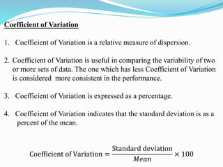
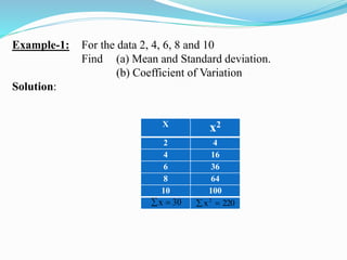
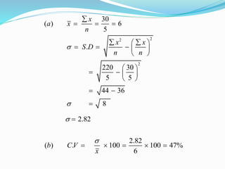
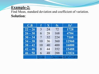
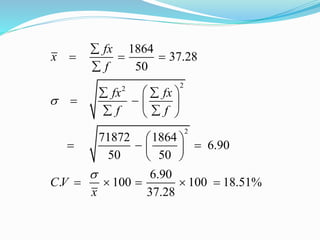
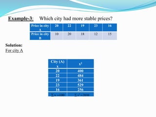
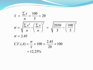
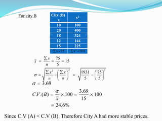
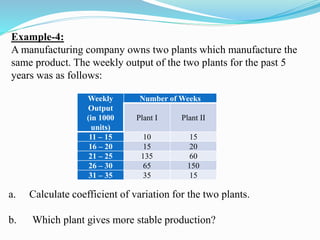
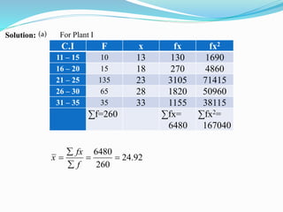
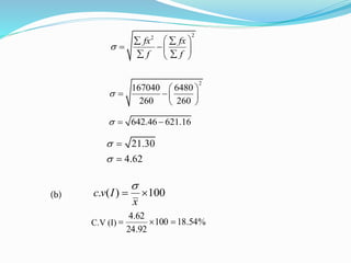
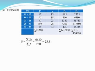
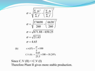
NADEEM UDDIN
ASSOCIATE PROFESSOR
OF STATISTICS
Coefficient of Variation
1. Coefficient of Variation is a relative measure of dispersion.
2. Coefficient of Variation is useful in comparing the variability of two
or more sets of data. The one which has less Coefficient of Variation
is considered more consistent in the performance.
3. Coefficient of Variation is expressed as a percentage.
4. Coefficient of Variation indicates that the standard deviation is as a
percent of the mean.
Coefficient of Variation =
Standard deviation
𝑀𝑒𝑎𝑛
× 100
Example-1: For the data 2, 4, 6, 8 and 10
Find (a) Mean and Standard deviation.
(b) Coefficient of Variation
Solution:
X
x2
2 4
4 16
6 36
8 64
10 100
30x  220x2

22
2
30
( ) 6
5
.
220 30
5 5
44 36
8
x
a x
n
x x
S D
n n



  
  
    
 
 
   
 
 

2.82 
2.82
( ) . 100 100 47%
6
b CV
x

    
C.B f X fx fx2
22 – 26 3 24 72 1728
26 – 30 6 28 168 4704
30 – 34 7 32 224 7168
34 – 38 10 36 360 12960
38 – 42 10 40 400 16000
42 – 46 8 44 352 15488
46 – 50 6 48 288 13824
50f  1864fx
2
71872fx 
Example-2:
Find Mean, standard deviation and coefficient of variation.
Solution:
22
2
1864
37.28
50
71872 1864
6.90
50 50
6.90
. 100 100 18.51%
37.28
fx
x
f
fx fx
f f
CV
x



  

  
   
  
 
   
 
    
Example-3: Which city had more stable prices?
Price in city
A
20 22 19 23 16
Price in city
B
10 20 18 12 15
Solution:
For city A
City (A)
x
x2
20 400
22 484
19 361
23 529
16 256
100x  2
2030x 
2 22
100
20
5
2030 100
5 5
2.45
2.45
. .( ) 100 100
20
12.25%
x
x
n
x x
n n
CV A
x




  
    
      
   

   

For city B City (B)
x
x2
10 100
20 400
18 324
12 144
15 225
75x  1931x2

2 22
75
15
5
1931 75
5 5
x
x
n
x x
n n


  
    
      
   
3.69
3.69
. .( ) 100 100
15
24.6%
C V B
x



   

Since C.V (A) < C.V (B). Therefore City A had more stable prices.
Example-4:
A manufacturing company owns two plants which manufacture the
same product. The weekly output of the two plants for the past 5
years was as follows:
Weekly
Output
(in 1000
units)
Number of Weeks
Plant I Plant II
11 – 15 10 15
16 – 20 15 20
21 – 25 135 60
26 – 30 65 150
31 – 35 35 15
a. Calculate coefficient of variation for the two plants.
b. Which plant gives more stable production?
Solution: For Plant I
C.I F x fx fx2
11 – 15 10 13 130 1690
16 – 20 15 18 270 4860
21 – 25 135 23 3105 71415
26 – 30 65 28 1820 50960
31 – 35 35 33 1155 38115
∑f=260 ∑fx=
6480
∑fx2=
167040
6480
24.92
260
fx
x
f

  

(a)
22
fx fx
f f

  
  
  
2
167040 6480
260 260

 
  
 
642.46 621.16  
21.30
4.62




. ( ) 100c v I
x

 
C.V (I) %54.18100
92.24
62.4

(b)
For Plant II
C.I F x fx fx2
11 – 15 15 13 195 2535
16 – 20 20 18 360 6480
21 – 25 60 23 1380 31740
26 – 30 150 28 4200 117600
31 – 35 15 33 495 16335
∑f=260 ∑fx=6630 ∑fx2=
174690
6630
25.5
260
fx
x
f

  

(a)
22
2
174690 6630
260 260
671.88 650.25
21.63
4.65
fx fx
f f





  
  
  
 
  
 
 


. ( ) 100c v II
x

 
C.V (II) %24.18100
5.25
65.4

Since C.V (II) < C.V (I)
Therefore Plant II gives more stable production.
(b)

Coefficient of variation

  • 1.
  • 2.
    Coefficient of Variation 1.Coefficient of Variation is a relative measure of dispersion. 2. Coefficient of Variation is useful in comparing the variability of two or more sets of data. The one which has less Coefficient of Variation is considered more consistent in the performance. 3. Coefficient of Variation is expressed as a percentage. 4. Coefficient of Variation indicates that the standard deviation is as a percent of the mean. Coefficient of Variation = Standard deviation 𝑀𝑒𝑎𝑛 × 100
  • 3.
    Example-1: For thedata 2, 4, 6, 8 and 10 Find (a) Mean and Standard deviation. (b) Coefficient of Variation Solution: X x2 2 4 4 16 6 36 8 64 10 100 30x  220x2 
  • 4.
    22 2 30 ( ) 6 5 . 22030 5 5 44 36 8 x a x n x x S D n n                            2.82  2.82 ( ) . 100 100 47% 6 b CV x      
  • 5.
    C.B f Xfx fx2 22 – 26 3 24 72 1728 26 – 30 6 28 168 4704 30 – 34 7 32 224 7168 34 – 38 10 36 360 12960 38 – 42 10 40 400 16000 42 – 46 8 44 352 15488 46 – 50 6 48 288 13824 50f  1864fx 2 71872fx  Example-2: Find Mean, standard deviation and coefficient of variation. Solution:
  • 6.
    22 2 1864 37.28 50 71872 1864 6.90 50 50 6.90 .100 100 18.51% 37.28 fx x f fx fx f f CV x                              
  • 7.
    Example-3: Which cityhad more stable prices? Price in city A 20 22 19 23 16 Price in city B 10 20 18 12 15 Solution: For city A City (A) x x2 20 400 22 484 19 361 23 529 16 256 100x  2 2030x 
  • 8.
    2 22 100 20 5 2030 100 55 2.45 2.45 . .( ) 100 100 20 12.25% x x n x x n n CV A x                             
  • 9.
    For city BCity (B) x x2 10 100 20 400 18 324 12 144 15 225 75x  1931x2  2 22 75 15 5 1931 75 5 5 x x n x x n n                      3.69 3.69 . .( ) 100 100 15 24.6% C V B x         Since C.V (A) < C.V (B). Therefore City A had more stable prices.
  • 10.
    Example-4: A manufacturing companyowns two plants which manufacture the same product. The weekly output of the two plants for the past 5 years was as follows: Weekly Output (in 1000 units) Number of Weeks Plant I Plant II 11 – 15 10 15 16 – 20 15 20 21 – 25 135 60 26 – 30 65 150 31 – 35 35 15 a. Calculate coefficient of variation for the two plants. b. Which plant gives more stable production?
  • 11.
    Solution: For PlantI C.I F x fx fx2 11 – 15 10 13 130 1690 16 – 20 15 18 270 4860 21 – 25 135 23 3105 71415 26 – 30 65 28 1820 50960 31 – 35 35 33 1155 38115 ∑f=260 ∑fx= 6480 ∑fx2= 167040 6480 24.92 260 fx x f      (a)
  • 12.
    22 fx fx f f          2 167040 6480 260 260         642.46 621.16   21.30 4.62     . ( ) 100c v I x    C.V (I) %54.18100 92.24 62.4  (b)
  • 13.
    For Plant II C.IF x fx fx2 11 – 15 15 13 195 2535 16 – 20 20 18 360 6480 21 – 25 60 23 1380 31740 26 – 30 150 28 4200 117600 31 – 35 15 33 495 16335 ∑f=260 ∑fx=6630 ∑fx2= 174690 6630 25.5 260 fx x f      (a)
  • 14.
    22 2 174690 6630 260 260 671.88650.25 21.63 4.65 fx fx f f                          . ( ) 100c v II x    C.V (II) %24.18100 5.25 65.4  Since C.V (II) < C.V (I) Therefore Plant II gives more stable production. (b)