Downloaded 69 times


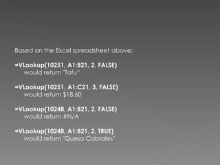
![ Looks in the first column of an array and moves
across the row to return the value of a cell
VLOOKUP(lookup_value, table_array,
col_index_num, [range_lookup])](https://image.slidesharecdn.com/lookupfunctions-120629082530-phpapp01/85/Look-up-functions-10-320.jpg)
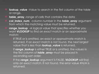
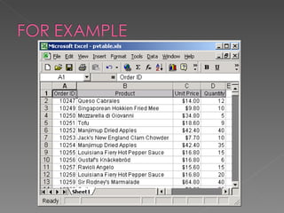

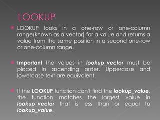
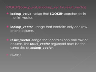
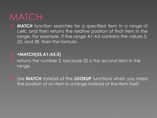
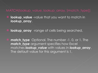
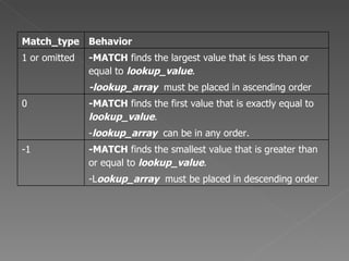
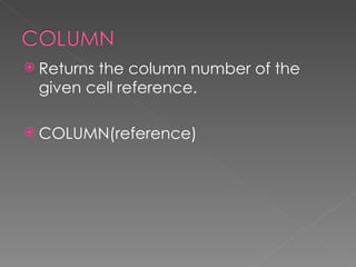
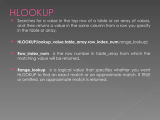
The document describes various lookup functions in Excel including LOOKUP, MATCH, HLOOKUP, VLOOKUP, COLUMN, and ROW. LOOKUP searches for a value in a one-column range and returns a value from the same position in a second range. MATCH returns the position of an item in a range. HLOOKUP and VLOOKUP search tables or arrays to return values, with HLOOKUP searching the top row and VLOOKUP the first column. COLUMN and ROW return the column or row number of a reference.