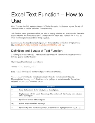
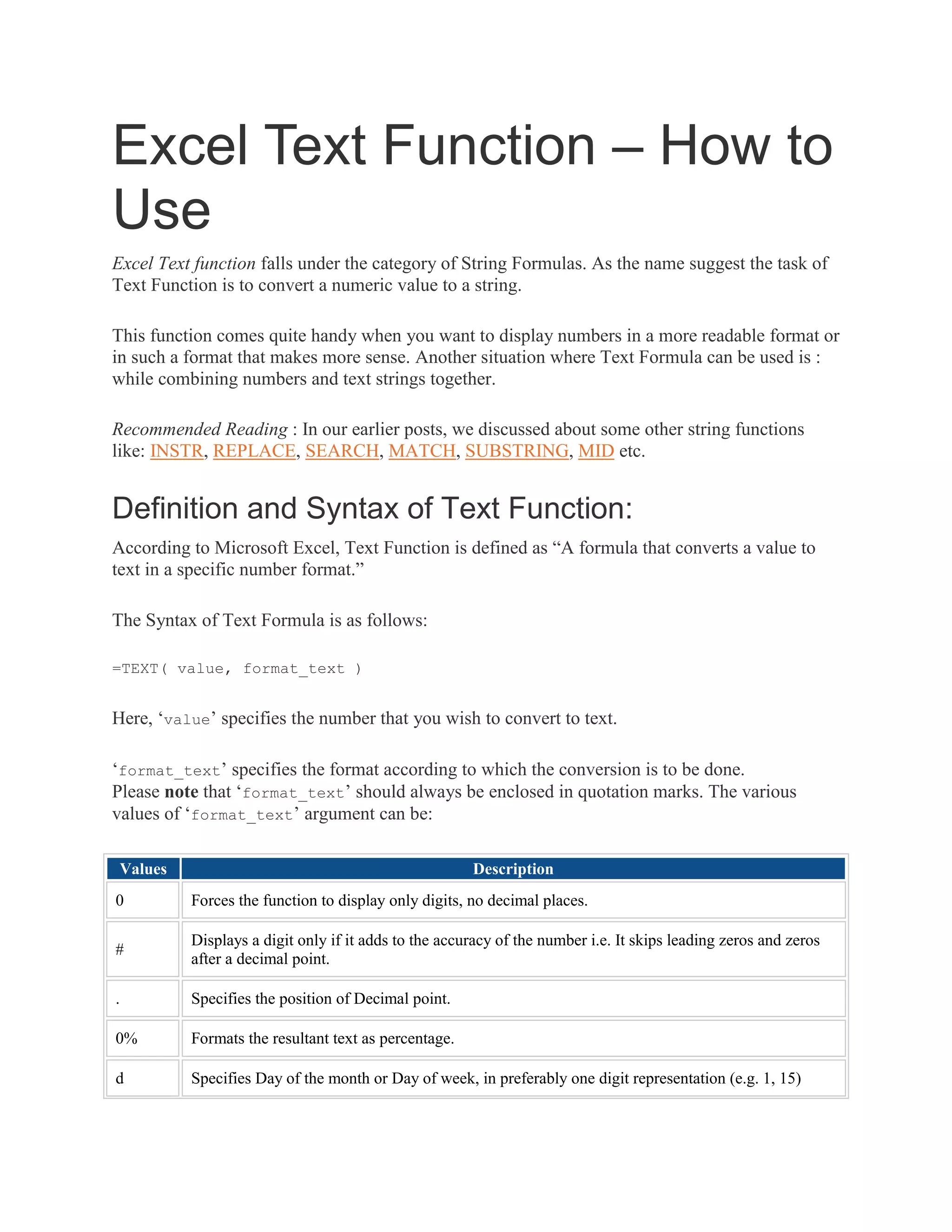
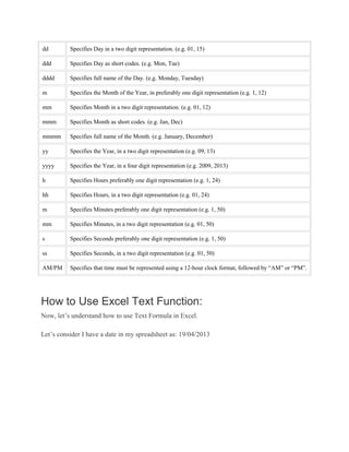
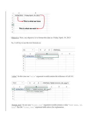
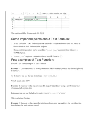
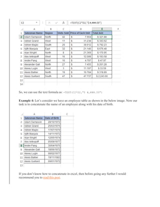
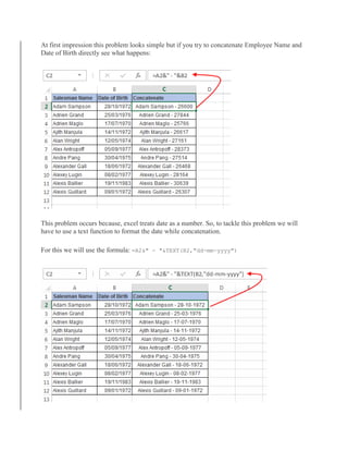
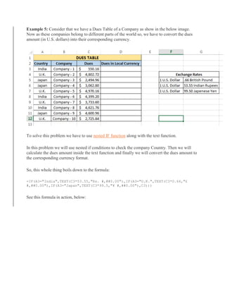
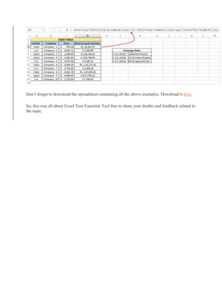
The Excel TEXT function converts numeric values to text strings in a specified format. It has two required arguments: the value to convert and the format text. The format text uses code like "0" or "dd-mm-yyyy" to determine how numbers or dates should be displayed as text. Some examples show using TEXT to format numbers with commas and currency symbols, concatenate text with formatted dates, and conditionally format values based on location. The TEXT function allows numbers to be displayed in readable formats and combined with text for reports.

1. Excel Text Function – How to
Use
Excel Text function falls under the category of String Formulas. As the name suggest the task of
Text Function is to convert a numeric value to a string.
This function comes quite handy when you want to display numbers in a more readable format or
in such a format that makes more sense. Another situation where Text Formula can be used is :
while combining numbers and text strings together.
Recommended Reading : In our earlier posts, we discussed about some other string functions
like: INSTR, REPLACE, SEARCH, MATCH, SUBSTRING, MID etc.
Definition and Syntax of Text Function:
According to Microsoft Excel, Text Function is defined as “A formula that converts a value to
text in a specific number format.”
The Syntax of Text Formula is as follows:
=TEXT( value, format_text )
Here, ‘value’ specifies the number that you wish to convert to text.
‘format_text’ specifies the format according to which the conversion is to be done.
Please note that ‘format_text’ should always be enclosed in quotation marks. The various
values of ‘format_text’ argument can be:
Values Description
0 Forces the function to display only digits, no decimal places.
#
Displays a digit only if it adds to the accuracy of the number i.e. It skips leading zeros and zeros
after a decimal point.
. Specifies the position of Decimal point.
0% Formats the resultant text as percentage.
d Specifies Day of the month or Day of week, in preferably one digit representation (e.g. 1, 15)

2. dd Specifies Day in a two digit representation. (e.g. 01, 15)
ddd Specifies Day as short codes. (e.g. Mon, Tue)
dddd Specifies full name of the Day. (e.g. Monday, Tuesday)
m Specifies the Month of the Year, in preferably one digit representation (e.g. 1, 12)
mm Specifies Month in a two digit representation. (e.g. 01, 12)
mmm Specifies Month as short codes. (e.g. Jan, Dec)
mmmm Specifies full name of the Month. (e.g. January, December)
yy Specifies the Year, in a two digit representation (e.g. 09, 13)
yyyy Specifies the Year, in a four digit representation (e.g. 2009, 2013)
h Specifies Hours preferably one digit representation (e.g. 1, 24)
hh Specifies Hours, in a two digit representation (e.g. 01, 24)
m Specifies Minutes preferably one digit representation (e.g. 1, 50)
mm Specifies Minutes, in a two digit representation (e.g. 01, 50)
s Specifies Seconds preferably one digit representation (e.g. 1, 50)
ss Specifies Seconds, in a two digit representation (e.g. 01, 50)
AM/PM Specifies that time must be represented using a 12-hour clock format, followed by “AM” or “PM”.
How to Use Excel Text Function:
Now, let’s understand how to use Text Formula in Excel.
Let’s consider I have a date in my spreadsheet as: 19/04/2013

3. Objective: Now, my objective is to format this date as: Friday April, 19, 2013
So, I will try to use the text formula as:
‘value’: In this case our ‘value’ argument would contain the reference of cell A1.
‘format_text’: In our case ‘format_text’ argument would contain a value “dddd mmmm, dd,
yyyy“. See the ‘format_text’ argument table above for explanation.

4. The result would be: Friday April, 19, 2013
Some Important points about Text Formula:
 As we know that TEXT formula converts a numeric value to formatted text, and hence its
result cannot be used for calculation purpose.
 If you omit the quotation marks around the ‘format_text’ argument then, it throws a
#NAME? error.
 ‘format_text’ argument cannot contain an asterisk character (*).
Few examples of Text Function:
Now let’s see some examples of Text Formula.
Example 1: Use text formula to display the nearest whole number (without any decimal places)
to 3390.34.
To do this we can use the text formula as: =TEXT(3390.34,0)
Which results into: 3390
Example 2: Suppose we have a date (say: 11-Aug-2013) and now using a text formula find
which day falls on that date.
In this case we can use the below formula: =TEXT("11-Aug-13","dddd")
This results into: Sunday
Example 3: Suppose we have a products table as shown, now we need to write a text function
that displays the total amount earned.

5. So, we can use the text formula as: =TEXT(C2*D2,"$ #,###.00")
Example 4: Let’s consider we have an employee table as shown in the below image. Now our
task is to concatenate the name of an employee along with his date of birth.
If you don’t know how to concatenate in excel, then before going any further I would
recommend you to read this post.

6. At first impression this problem looks simple but if you try to concatenate Employee Name and
Date of Birth directly see what happens:
This problem occurs because, excel treats date as a number. So, to tackle this problem we will
have to use a text function to format the date while concatenation.
For this we will use the formula: =A2&" - "&TEXT(B2,"dd-mm-yyyy")

7. Example 5: Consider that we have a Dues Table of a Company as show in the below image.
Now as these companies belong to different parts of the world so, we have to convert the dues
amount (in U.S. dollars) into their corresponding currency.
To solve this problem we have to use nested IF function along with the text function.
In this problem we will use nested if conditions to check the company Country. Then we will
calculate the dues amount inside the text function and finally we will convert the dues amount to
the corresponding currency format.
So, this whole thing boils down to the formula:
=IF(A3="India",TEXT(C3*53.55,"Rs. #,##0.00"),IF(A3="U.K.",TEXT(C3*0.66,"£
#,##0.00"),IF(A3="Japan",TEXT(C3*99.5,"¥ #,##0.00"),C3)))
See this formula in action, below:

8. Don’t forget to download the spreadsheet containing all the above examples. Download it here.
So, this was all about Excel Text Function. Feel free to share your doubts and feedback related to
the topic.