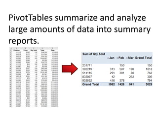
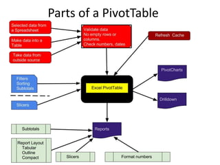
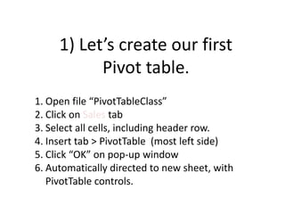
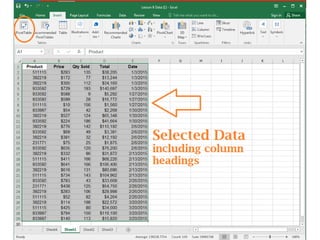
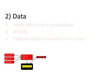
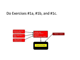
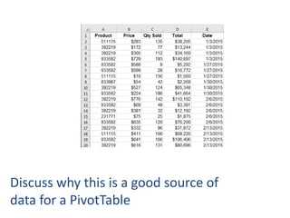
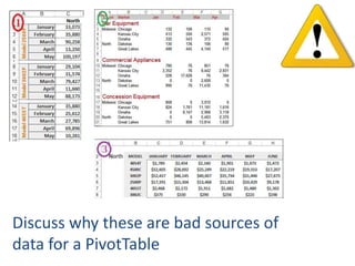
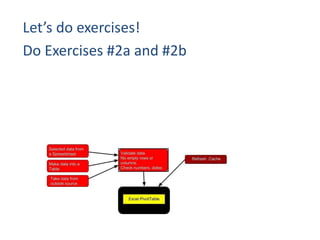
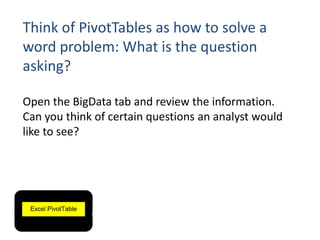
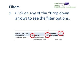
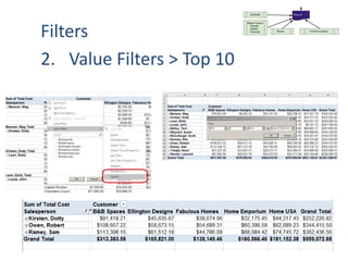
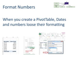
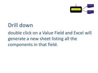
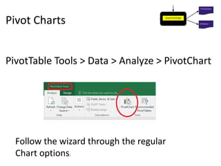
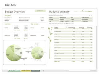
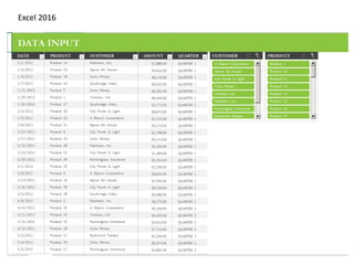
DISCOVER . LEARN .
EMPOWER
Topic of
Presentation:
Research
Process Steps
INSTITUTE –University
School of Business
DEPARTMENT -Management
M.B.A
Marketing Analytics- 21BAT757
Ms. Simmi Dhyani
Assistant Professor
1
PivotTables summarize and analyze
large amounts of data into summary
reports.
Parts of a PivotTable
1) Let’s create our first
Pivot table.
1. Open file “PivotTableClass”
2. Click on Sales tab
3. Select all cells, including header row.
4. Insert tab > PivotTable (most left side)
5. Click “OK” on pop-up window
6. Automatically directed to new sheet, with
PivotTable controls.
The Create PivotTable Dialog box.
The address of the data we just selected appears
here.
Most frequently we put the new PivotTable on an
new worksheet.
Click OK
The ribbon for PivotTables
Parts of a PivotTable
Excel
2016
Input to a PivotTable
A closer view:
2) Data
1. Select data from a spreadsheet
2. A Table
3. External Data (not covered in this class)
1. Select data from a spreadsheet
• Click on upper left part of
data, including the column
heading.
• Press Shift key.
• Click on lower right cell of
data.
• Release Shift key.
2. Create a table from data
• Select all the desired cells
• Insert tab > Table
• Click “OK” on the Create Table
dialog box.
• Note the Name Box – it now
has Table1 in it.
When you create a PivotTable, a copy of the
data is stored in a pivot cache. Any changes
to the data won’t show up in the report
until you refresh the cache.
To refresh the data:
• Right-click the pivot table and click Refresh Data. Or
• Go to the Options tab, and click the Refresh button
Do Exercises #1a, #1b, and #1c.
The data needs to be clean.
Any blank rows, blank columns, or text in a
number field will give unpredictable results.
Ex: Summing a number field with blanks
becomes a Count.
Use Conditional formatting on
number fields to search for invalid
data.
Find invalid numbers
1. Select a column or range of cells.
2. Home > Conditional Formatting
The data :
• Must have Column Headings in the first
row.
• Must have tabular layout - no blank rows
or columns.
• No repeating columns of data
Normalized data
Discuss why this is a good source of
data for a PivotTable
Discuss why these are bad sources of
data for a PivotTable
Let’s do exercises!
Do Exercises #2a and #2b
Think of PivotTables as how to solve a
word problem: What is the question
asking?
Open the BigData tab and review the information.
Can you think of certain questions an analyst would
like to see?
Subtotals
PivotTable Tools > Design >Layout
Subtotals control allows you to toggle
subtotals on and off, as well as place them at
the top or bottom of the section.
Tabular
Report options:
Compact
Outline
There are at least two ways of
selecting / limiting data:
 Filters
 Slicers
Slicers
Interactive, good for doing “what-if”
scenarios
Filters
1. Click on any of the “Drop down
arrows to see the filter options.
Filters
2. Value Filters > Top 10
Format Numbers
When you create a PivotTable, Dates
and numbers loose their formatting
Drill down
double click on a Value Field and Excel will
generate a new sheet listing all the
components in that field.
Pivot Charts
PivotTable Tools > Data > Analyze > PivotChart
Follow the wizard through the regular
Chart options.
Excel 2016
Excel 2016
Thank You

Excel and Pivot Tables.pptx

  • 1.
    DISCOVER . LEARN. EMPOWER Topic of Presentation: Research Process Steps INSTITUTE –University School of Business DEPARTMENT -Management M.B.A Marketing Analytics- 21BAT757 Ms. Simmi Dhyani Assistant Professor 1
  • 2.
    PivotTables summarize andanalyze large amounts of data into summary reports.
  • 3.
    Parts of aPivotTable
  • 4.
    1) Let’s createour first Pivot table. 1. Open file “PivotTableClass” 2. Click on Sales tab 3. Select all cells, including header row. 4. Insert tab > PivotTable (most left side) 5. Click “OK” on pop-up window 6. Automatically directed to new sheet, with PivotTable controls.
  • 6.
    The Create PivotTableDialog box. The address of the data we just selected appears here. Most frequently we put the new PivotTable on an new worksheet. Click OK
  • 8.
    The ribbon forPivotTables
  • 9.
    Parts of aPivotTable Excel 2016
  • 10.
    Input to aPivotTable A closer view:
  • 11.
    2) Data 1. Selectdata from a spreadsheet 2. A Table 3. External Data (not covered in this class)
  • 12.
    1. Select datafrom a spreadsheet • Click on upper left part of data, including the column heading. • Press Shift key. • Click on lower right cell of data. • Release Shift key.
  • 13.
    2. Create atable from data • Select all the desired cells • Insert tab > Table • Click “OK” on the Create Table dialog box. • Note the Name Box – it now has Table1 in it.
  • 14.
    When you createa PivotTable, a copy of the data is stored in a pivot cache. Any changes to the data won’t show up in the report until you refresh the cache. To refresh the data: • Right-click the pivot table and click Refresh Data. Or • Go to the Options tab, and click the Refresh button
  • 15.
    Do Exercises #1a,#1b, and #1c.
  • 16.
    The data needsto be clean. Any blank rows, blank columns, or text in a number field will give unpredictable results. Ex: Summing a number field with blanks becomes a Count. Use Conditional formatting on number fields to search for invalid data.
  • 17.
    Find invalid numbers 1.Select a column or range of cells. 2. Home > Conditional Formatting
  • 18.
    The data : •Must have Column Headings in the first row. • Must have tabular layout - no blank rows or columns. • No repeating columns of data Normalized data
  • 19.
    Discuss why thisis a good source of data for a PivotTable
  • 20.
    Discuss why theseare bad sources of data for a PivotTable
  • 21.
    Let’s do exercises! DoExercises #2a and #2b
  • 22.
    Think of PivotTablesas how to solve a word problem: What is the question asking? Open the BigData tab and review the information. Can you think of certain questions an analyst would like to see?
  • 23.
    Subtotals PivotTable Tools >Design >Layout Subtotals control allows you to toggle subtotals on and off, as well as place them at the top or bottom of the section.
  • 24.
  • 25.
    There are atleast two ways of selecting / limiting data:  Filters  Slicers
  • 26.
    Slicers Interactive, good fordoing “what-if” scenarios
  • 27.
    Filters 1. Click onany of the “Drop down arrows to see the filter options.
  • 28.
  • 29.
    Format Numbers When youcreate a PivotTable, Dates and numbers loose their formatting
  • 30.
    Drill down double clickon a Value Field and Excel will generate a new sheet listing all the components in that field.
  • 31.
    Pivot Charts PivotTable Tools> Data > Analyze > PivotChart Follow the wizard through the regular Chart options.
  • 32.
  • 33.
  • 34.