Downloaded 337 times
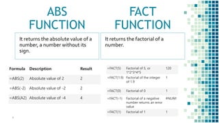
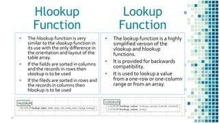
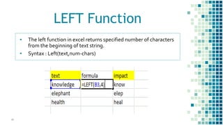
![SUMIF Function
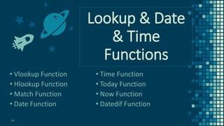
▪ You use the SUMIF
function to sum the values
in a range that meet
criteria that you specify.
▪ For example, suppose that
in a column that contains
numbers, you want to sum
only the values that are
larger than 5.You can use
the following formula:
=SUMIF(B2:B25,">5")
▪ Syntax : SUMIF(range,
criteria, [sum_range])
8](https://image.slidesharecdn.com/51-56-morning-usingexcelfunctionincaprofession-180324072935/85/Using-Excel-Functions-8-320.jpg)
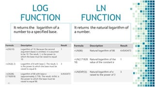
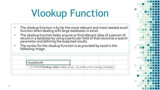
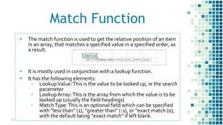
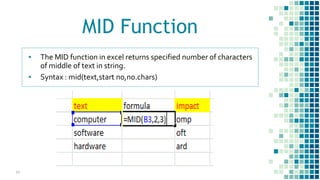
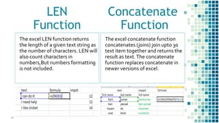
![MAX
FUNCTION
Max function returns the largest
value in a set of values.
SYNTAX:
MAX(number1,[number2],….)|:
Median function returns the median, or
the number in the middle of the set of
given numbers.
SYNTAX :
MEDIAN(number1,[number2],….)
MEDIAN
FUNCTION
16](https://image.slidesharecdn.com/51-56-morning-usingexcelfunctionincaprofession-180324072935/85/Using-Excel-Functions-16-320.jpg)
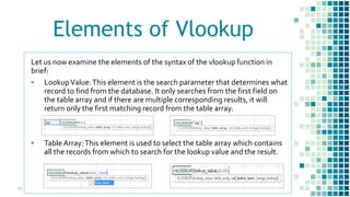
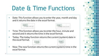
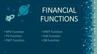
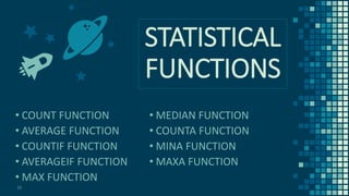
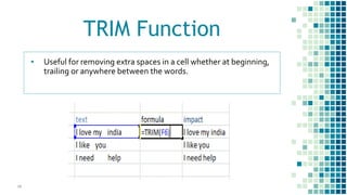
![FV (Future Value)
▪ It calculates future value of an
investment based on periodic,
constant payments and a constant
interest rate.
▪ Syntax : FV(rate, nper ,pmt
,[pv],[type])
▪ Where,
▫ Rate = interest rate per period
▫ Nper = total no. of payment
periods.
▫ Pmt = payment made each
period.
▫ [pv] = present value of series of
future payments.
▫ [type] = indicates when
payment is due.
▫ 0 = at the end of a period
▫ 1 = at the beg. of a period28](https://image.slidesharecdn.com/51-56-morning-usingexcelfunctionincaprofession-180324072935/85/Using-Excel-Functions-28-320.jpg)
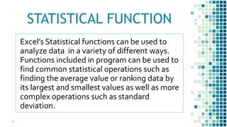
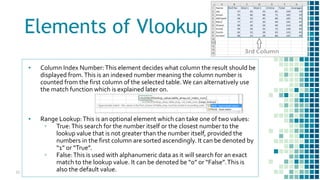
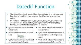
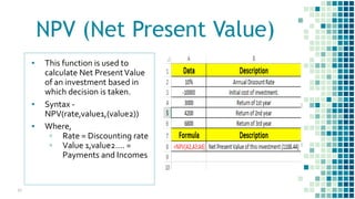
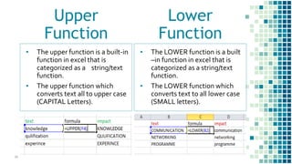
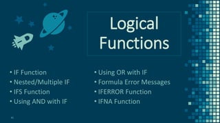
![IRR (Internal Rate of Return)
▪ It calculates the internal rate of
return for a series of cash flows
represented by the number in
values.
▪ Syntax - Irr(values,[guess])
▪ Where,
▫ Values = reference to cells
that contain no.s for which
irr is calculated.
▫ Guess = it is a no. user
guesses to be close to the
result of irr.
29](https://image.slidesharecdn.com/51-56-morning-usingexcelfunctionincaprofession-180324072935/85/Using-Excel-Functions-29-320.jpg)
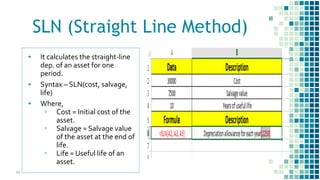
![DB (DIMINISHING VALUE
METHOD)
▪ It calculates dep. byWritten
DownValue method for one
period.
▪ Syntax – DB(cost, salvage, life,
period, [factor]
▪ Where,
▫ Cost = Initial cost of an
asset.
▫ Salvage = Salvage value at
the of life of asset.
▫ Life = Useful life of asset.
▫ Period = Period for which
depreciation is calculated.
31](https://image.slidesharecdn.com/51-56-morning-usingexcelfunctionincaprofession-180324072935/85/Using-Excel-Functions-31-320.jpg)
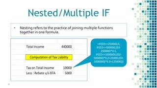
![PMT (PAYMENT PER PERIOD)
▪ It calculates the payment for
a loan based on constant
payments and constant
interest rate.
▪ Syntax –Pmt(rate, nper, pv,
[fv],[type])
▪ Where,
▫ Rate = rate of interest
per period
▫ Nper = no, of payments
for the loan.
▫ Pv = Principal.
32](https://image.slidesharecdn.com/51-56-morning-usingexcelfunctionincaprofession-180324072935/85/Using-Excel-Functions-32-320.jpg)
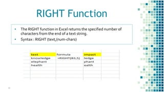
![IPMT (INTEREST PER PERIOD)
▪ Used to calculate interest earned
on various recurring investments.
▪ Syntax : Ipmt(rate, per, nper, pv,
[fv], [type])
▪ Where,
▫ Rate = interest rate per
period.
▫ Per = it is the period for
which interest is calculated.
▫ Nper = total no. of payment
period.
▫ Pv = amount invested in
lumpsum.
33](https://image.slidesharecdn.com/51-56-morning-usingexcelfunctionincaprofession-180324072935/85/Using-Excel-Functions-33-320.jpg)

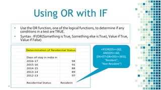
![IF Function
▪ Checks whether a condition is met, and returns one value if
TRUE, and another value if FALSE.
▪ Syntax : IF(logical_test, [value_if_true], [value_if_false])
=IF(D1<=500000,5000,0)
42](https://image.slidesharecdn.com/51-56-morning-usingexcelfunctionincaprofession-180324072935/85/Using-Excel-Functions-42-320.jpg)
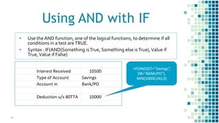
![IFS Function (Excel 2016)
▪ There is now an IFS function that can replace multiple, nested IF
statements with a single function.
▪ Syntax : IFS(condition1, value1, [condition2], [value2], [condition3],
[value3], …)
=IFS(D2<=250000,0,
D2<=500000,(D2-
250000)*0.1,
D2<=1000000,(D2-
500000)*0.2+25000,
true,(D2-1000000)*0.3
+125000)
44](https://image.slidesharecdn.com/51-56-morning-usingexcelfunctionincaprofession-180324072935/85/Using-Excel-Functions-44-320.jpg)


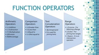
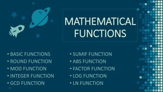
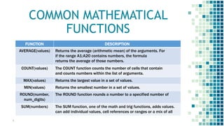
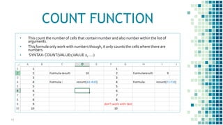
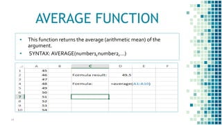
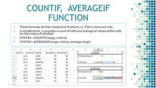
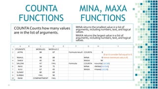
The document provides an overview of various Excel functions organized into categories including: 1. Mathematical functions such as ROUND, MOD, INTEGER, GCD, and LOG functions. 2. Statistical functions such as COUNT, AVERAGE, MAX, MEDIAN, and financial functions such as NPV, PV, PMT. 3. Lookup functions including VLOOKUP, HLOOKUP, MATCH to find data in tables or perform lookups. 4. Date and time functions like DATE, TIME, TODAY, NOW and DATEDIF to work with dates and times. 5. Text functions including LEFT, RIGHT, MID, UPPER, LOWER, LEN to manipulate