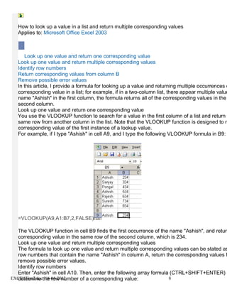
Samples:

=IF(ISNA(VLOOKUP(A3,PostCodeFull!
$A$3:$G$25000,7,FALSE)),0,VLOOKUP(A3,PostCodeFull!
$A$3:$G$25000,7,FALSE))

=IF(ISNA(VLOOKUP(P3,Addressbook!$A$3:$G$25000,7,FALSE)),0,VLOOKUP(P3,
Addressbook !$A$3:$G$25000,7,FALSE))

=IF(ISNA(VLOOKUP($B3,CostAve02!$A$3:$I$65000,9,FALSE)),"No
Cost",VLOOKUP($B3, CostAve02!$A$3:$I$65000,9,FALSE))

=IF(ISNA(VLOOKUP(P3,Addressbook!
(A3:E2000,3,FALSE)),"Missing",A3,VLOOKUP(Addressbook!(P3,A3:E20000,3,FALSE)))

Check data type, numeric to numeric column or text to text type data


1Problem:

Column B contains values to look up in List1 (Column A).
How could we alter the results returned by the VLOOKUP function so that they will
include the original value looked up and a ""Found""/""Not Found"" indication?

1.Solution:

Use the ISNA and VLOOKUP functions in an IF statement, as follows:
=IF(ISNA(VLOOKUP(B2,$A$2:$A$7,1,FALSE)),B2&"" Not
Found"",VLOOKUP(B2,$A$2:$A$7,1,FALSE)&"" Found"")


List1_____Values to look______Result
Blue______Pink________________Pink Not Found
Red_______Blue________________Blue Found
Green_____White_______________White Not Found
Black_____Purple______________Purple Not Found
Yellow____Red_________________Red Found
Orange

Problem:

Columns A & B contain two lists of values.
We want to create a formula that will check whether there is any duplication of

EXCELTips2.doc 18-04-2012                                              1
values within either list (blank cells are to be ignored).

Solution:

Use the COUNTA, SUMPRODUCT, and COUNTIF functions as shown in the following
formula:
=IF(COUNTA(A2:A7)=SUMPRODUCT((A2:A7<>"")/COUNTIF(A2:A7,A2:A7&"")),"No
Duplicates","Duplicates")
The formula will return "Duplicates" if the list contains duplicate values, otherwise it will
return "No Duplicates".


List1____List2
1________1
2
3________B
A________2
________3
1________4


Problem:

Column B in sheet1 contains numbers. Columns B:C in sheet2 contain numbers
and their matching text.
How could we find the text in sheet2 matching each number in sheet1?

Solution:

The following formula will find the text in sheet2 matching to the number in cell B13 in
sheet1:
=IF(ISNA(VLOOKUP(B13,$B$20:$B$24,1,FALSE)),"Not
Found",VLOOKUP(B13,$B$20:$C$24,2,FALSE))
In case the number is not found in sheet2, using ISNA function, the formula will return
Not Found.

Example:

Sheet1

Number__Result_______Formula
1_______One__________=IF(ISNA(VLOOKUP(B13,$B$20:$B$24,1,FALSE)),"Not
Found",VLOOKUP(B13,$B$20:$C$24,2,FALSE((
EXCELTips2.doc 18-04-2012                                                2
9_______Not Found____=IF(ISNA(VLOOKUP(B14,$B$20:$B$24,1,FALSE)),"Not
Found",VLOOKUP(B14,$B$20:$C$24,2,FALSE((
3_______Three________=IF(ISNA(VLOOKUP(B15,$B$20:$B$24,1,FALSE)),"Not
Found",VLOOKUP(B15,$B$20:$C$24,2,FALSE))


Sheet2

Number__Text
4_______Four
5_______Five
3_______Three
6_______Six
1_______One

To eliminate errors that occur when using the Vlookup Formula:

In the screenshot below are four Vlookup Formulas. In this example, we asume that the
index number 1346 is not included in the index list in the leftmost column of the data
table, the index number 1353 is included and the defined Name for the data table is Data:

Cell C2: The fourth argument of the Vlookup Formula is empty, therefore, the formula
returns a result according to a number equal to or less than the lookup number from the
index list.

Cell C4: In the fourth argument of the Vlookup Formula = FALSE, therefore, the formula
returns errors when the lookup value is not included in the index list, which is the leftmost
column of the data table.

Cell C6: The ISERROR formula, nested in the IF formula, returns TRUE when Vlookup
Formula returns an error, and therefore, the final result is 0.

Cell C8: The ISERROR formula nested in the IF formula returns FALSE and the Vlookup
formula returns the appropriate result number.

Problem:

Columns C & D contain pairs of row and column numbers representing some of
the cells in Data Range (A2:B5).
We want to create a cell reference from each pair of numbers in columns C & D and
then retrieve the value stored in that cell.

Solution:

EXCELTips2.doc 18-04-2012                                              3
"Use the INDIRECT and ADDRESS functions as shown in the following formula:
=INDIRECT(ADDRESS(C2,D2))

Problem:

Range1 (A3:C7) contains file names with their matching types and sizes.
Range2 (A12:B16) contains a similar list of file names but with matching types only.
We want to find the appropriate file sizes from Range1 by matching each pair of file
names and types from both ranges.

Solution:

Use the INDEX and MATCH functions as shown in the following formula:
{=INDEX($C$3:$C$7,MATCH(A12&B12,$A$3:$A$7&$B$3:$B$7,0))}

(To create Array formula: select the cell after typing the formula,press F2 and then press
Ctrl+Shift+Enter)

Example:

Range1

File Name_______File Type_______Size (KB)
file1___________xls_____________500
file2___________doc_____________80
file3___________ppt_____________800
file4___________xls_____________400
file1___________ppt_____________1200


Range2

File Name_____________File Type_____________Size (KB) from Range1
file1_________________xls___________________500
file2_________________doc___________________80
file3_________________ppt___________________800
file4_________________xls___________________400
file1_________________ppt___________________1200

Problem:

Retrieving the matching price of the item shown in cell A2, for the specific brand
entered in cell B2.

EXCELTips2.doc 18-04-2012                                             4
Following are the prices for each possible combination:
Item,Brand,Price
Jeans, Diesel, $85
Jeans, Levis, $80
Jeans, Lee, $70
T-Shirt, Sacks, $7
T-Shirt, Gap, $5
T-Shirt, Old Navy, $3

Solution:

Use the IF and LOOKUP functions as shown in the following formula:
=IF(A2="Jeans",LOOKUP(B2,{"Diesel","Lee","Levis";85,70,80}),IF(A2="T-
Shirt",LOOKUP(B2,{"Gap","Old Navy","Sacks"},{5,3,7})))

Problem:

Column B contains the mark matching each of the grades shown in column A.
We want to grade each mark in column D by finding the mark closest to it in
column B, and then retrieving the corresponding grade from column A.

Solution:

Use the INDEX, MIN, IF, ABS, and ROW functions as shown in the following Array
formula:
{=INDEX($A$2:$A$6,MIN(IF(ABS($B$2:$B$6-D2)=MIN(ABS($B$2:$B$6-
D2)),ROW($B$2:$B$6)-ROW($B$2)+1)),1)}

To apply Array formula:
Select the cell, press and simultaneously press .

Problem:

Listed in range1 (A4:B6) and range2 (D4:E6) are clothing items and their prices.
Cell B9 contains the name of an item from one of the ranges.
We would like to perform a lookup on both ranges, find the relevant item, and
return the matching price.

Solution:

Use the ISNA and VLOOKUP functions as shown in the following formula:


EXCELTips2.doc 18-04-2012                                        5
=IF(ISNA(VLOOKUP(B9,A4:B6,2,FALSE)),VLOOKUP(B9,D4:E6,2,FALSE),VLOOKUP(B
9,A4:B6,2,FALSE))

Problem:

Columns A & B list all the pay dates of various clients.
We want to retrieve the date of the most recent payment made by each of the
clients listed in column D.

Solution:

Use the MAX and IF functions as shown in the following Array formula:
{=MAX(IF($A$2:$A$8=D2,$B$2:$B$8))}


EXCELTips2.doc 18-04-2012                                          6
EXCELTips2.doc 18-04-2012   7
How to look up a value in a list and return multiple corresponding values
   Applies to: Microsoft Office Excel 2003


      Look up one value and return one corresponding value
   Look up one value and return multiple corresponding values
   Identify row numbers
   Return corresponding values from column B
   Remove possible error values
   In this article, I provide a formula for looking up a value and returning multiple occurrences o
   corresponding value in a list; for example, if in a two-column list, there appear multiple value
   name "Ashish" in the first column, the formula returns all of the corresponding values in the
   second column.
   Look up one value and return one corresponding value
   You use the VLOOKUP function to search for a value in the first column of a list and return a
   same row from another column in the list. Note that the VLOOKUP function is designed to re
   corresponding value of the first instance of a lookup value.
   For example, if I type "Ashish" in cell A9, and I type the following VLOOKUP formula in B9:


   =VLOOKUP(A9,A1:B7,2,FALSE)

  The VLOOKUP function in cell B9 finds the first occurrence of the name "Ashish", and return
  corresponding value in the same row of the second column, which is 234.
  Look up one value and return multiple corresponding values
  The formula to look up one value and return multiple corresponding values can be stated as
  row numbers that contain the name "Ashish" in column A, return the corresponding values f
  remove possible error values.
  Identify row numbers
  Enter "Ashish" in cell A10. Then, enter the following array formula (CTRL+SHIFT+ENTER) i
EXCELTips2.docthe row number of a corresponding value:
  determine 18-04-2012                                               8
EXCELTips2.doc 18-04-2012   9

Excel tips

  • 1.
    Samples: =IF(ISNA(VLOOKUP(A3,PostCodeFull! $A$3:$G$25000,7,FALSE)),0,VLOOKUP(A3,PostCodeFull! $A$3:$G$25000,7,FALSE)) =IF(ISNA(VLOOKUP(P3,Addressbook!$A$3:$G$25000,7,FALSE)),0,VLOOKUP(P3, Addressbook !$A$3:$G$25000,7,FALSE)) =IF(ISNA(VLOOKUP($B3,CostAve02!$A$3:$I$65000,9,FALSE)),"No Cost",VLOOKUP($B3, CostAve02!$A$3:$I$65000,9,FALSE)) =IF(ISNA(VLOOKUP(P3,Addressbook! (A3:E2000,3,FALSE)),"Missing",A3,VLOOKUP(Addressbook!(P3,A3:E20000,3,FALSE))) Checkdata type, numeric to numeric column or text to text type data 1Problem: Column B contains values to look up in List1 (Column A). How could we alter the results returned by the VLOOKUP function so that they will include the original value looked up and a ""Found""/""Not Found"" indication? 1.Solution: Use the ISNA and VLOOKUP functions in an IF statement, as follows: =IF(ISNA(VLOOKUP(B2,$A$2:$A$7,1,FALSE)),B2&"" Not Found"",VLOOKUP(B2,$A$2:$A$7,1,FALSE)&"" Found"") List1_____Values to look______Result Blue______Pink________________Pink Not Found Red_______Blue________________Blue Found Green_____White_______________White Not Found Black_____Purple______________Purple Not Found Yellow____Red_________________Red Found Orange Problem: Columns A & B contain two lists of values. We want to create a formula that will check whether there is any duplication of EXCELTips2.doc 18-04-2012 1
  • 2.
    values within eitherlist (blank cells are to be ignored). Solution: Use the COUNTA, SUMPRODUCT, and COUNTIF functions as shown in the following formula: =IF(COUNTA(A2:A7)=SUMPRODUCT((A2:A7<>"")/COUNTIF(A2:A7,A2:A7&"")),"No Duplicates","Duplicates") The formula will return "Duplicates" if the list contains duplicate values, otherwise it will return "No Duplicates". List1____List2 1________1 2 3________B A________2 ________3 1________4 Problem: Column B in sheet1 contains numbers. Columns B:C in sheet2 contain numbers and their matching text. How could we find the text in sheet2 matching each number in sheet1? Solution: The following formula will find the text in sheet2 matching to the number in cell B13 in sheet1: =IF(ISNA(VLOOKUP(B13,$B$20:$B$24,1,FALSE)),"Not Found",VLOOKUP(B13,$B$20:$C$24,2,FALSE)) In case the number is not found in sheet2, using ISNA function, the formula will return Not Found. Example: Sheet1 Number__Result_______Formula 1_______One__________=IF(ISNA(VLOOKUP(B13,$B$20:$B$24,1,FALSE)),"Not Found",VLOOKUP(B13,$B$20:$C$24,2,FALSE(( EXCELTips2.doc 18-04-2012 2
  • 3.
    9_______Not Found____=IF(ISNA(VLOOKUP(B14,$B$20:$B$24,1,FALSE)),"Not Found",VLOOKUP(B14,$B$20:$C$24,2,FALSE(( 3_______Three________=IF(ISNA(VLOOKUP(B15,$B$20:$B$24,1,FALSE)),"Not Found",VLOOKUP(B15,$B$20:$C$24,2,FALSE)) Sheet2 Number__Text 4_______Four 5_______Five 3_______Three 6_______Six 1_______One To eliminateerrors that occur when using the Vlookup Formula: In the screenshot below are four Vlookup Formulas. In this example, we asume that the index number 1346 is not included in the index list in the leftmost column of the data table, the index number 1353 is included and the defined Name for the data table is Data: Cell C2: The fourth argument of the Vlookup Formula is empty, therefore, the formula returns a result according to a number equal to or less than the lookup number from the index list. Cell C4: In the fourth argument of the Vlookup Formula = FALSE, therefore, the formula returns errors when the lookup value is not included in the index list, which is the leftmost column of the data table. Cell C6: The ISERROR formula, nested in the IF formula, returns TRUE when Vlookup Formula returns an error, and therefore, the final result is 0. Cell C8: The ISERROR formula nested in the IF formula returns FALSE and the Vlookup formula returns the appropriate result number. Problem: Columns C & D contain pairs of row and column numbers representing some of the cells in Data Range (A2:B5). We want to create a cell reference from each pair of numbers in columns C & D and then retrieve the value stored in that cell. Solution: EXCELTips2.doc 18-04-2012 3
  • 4.
    "Use the INDIRECTand ADDRESS functions as shown in the following formula: =INDIRECT(ADDRESS(C2,D2)) Problem: Range1 (A3:C7) contains file names with their matching types and sizes. Range2 (A12:B16) contains a similar list of file names but with matching types only. We want to find the appropriate file sizes from Range1 by matching each pair of file names and types from both ranges. Solution: Use the INDEX and MATCH functions as shown in the following formula: {=INDEX($C$3:$C$7,MATCH(A12&B12,$A$3:$A$7&$B$3:$B$7,0))} (To create Array formula: select the cell after typing the formula,press F2 and then press Ctrl+Shift+Enter) Example: Range1 File Name_______File Type_______Size (KB) file1___________xls_____________500 file2___________doc_____________80 file3___________ppt_____________800 file4___________xls_____________400 file1___________ppt_____________1200 Range2 File Name_____________File Type_____________Size (KB) from Range1 file1_________________xls___________________500 file2_________________doc___________________80 file3_________________ppt___________________800 file4_________________xls___________________400 file1_________________ppt___________________1200 Problem: Retrieving the matching price of the item shown in cell A2, for the specific brand entered in cell B2. EXCELTips2.doc 18-04-2012 4
  • 5.
    Following are theprices for each possible combination: Item,Brand,Price Jeans, Diesel, $85 Jeans, Levis, $80 Jeans, Lee, $70 T-Shirt, Sacks, $7 T-Shirt, Gap, $5 T-Shirt, Old Navy, $3 Solution: Use the IF and LOOKUP functions as shown in the following formula: =IF(A2="Jeans",LOOKUP(B2,{"Diesel","Lee","Levis";85,70,80}),IF(A2="T- Shirt",LOOKUP(B2,{"Gap","Old Navy","Sacks"},{5,3,7}))) Problem: Column B contains the mark matching each of the grades shown in column A. We want to grade each mark in column D by finding the mark closest to it in column B, and then retrieving the corresponding grade from column A. Solution: Use the INDEX, MIN, IF, ABS, and ROW functions as shown in the following Array formula: {=INDEX($A$2:$A$6,MIN(IF(ABS($B$2:$B$6-D2)=MIN(ABS($B$2:$B$6- D2)),ROW($B$2:$B$6)-ROW($B$2)+1)),1)} To apply Array formula: Select the cell, press and simultaneously press . Problem: Listed in range1 (A4:B6) and range2 (D4:E6) are clothing items and their prices. Cell B9 contains the name of an item from one of the ranges. We would like to perform a lookup on both ranges, find the relevant item, and return the matching price. Solution: Use the ISNA and VLOOKUP functions as shown in the following formula: EXCELTips2.doc 18-04-2012 5
  • 6.
    =IF(ISNA(VLOOKUP(B9,A4:B6,2,FALSE)),VLOOKUP(B9,D4:E6,2,FALSE),VLOOKUP(B 9,A4:B6,2,FALSE)) Problem: Columns A &B list all the pay dates of various clients. We want to retrieve the date of the most recent payment made by each of the clients listed in column D. Solution: Use the MAX and IF functions as shown in the following Array formula: {=MAX(IF($A$2:$A$8=D2,$B$2:$B$8))} EXCELTips2.doc 18-04-2012 6
  • 7.
  • 8.
    How to lookup a value in a list and return multiple corresponding values Applies to: Microsoft Office Excel 2003 Look up one value and return one corresponding value Look up one value and return multiple corresponding values Identify row numbers Return corresponding values from column B Remove possible error values In this article, I provide a formula for looking up a value and returning multiple occurrences o corresponding value in a list; for example, if in a two-column list, there appear multiple value name "Ashish" in the first column, the formula returns all of the corresponding values in the second column. Look up one value and return one corresponding value You use the VLOOKUP function to search for a value in the first column of a list and return a same row from another column in the list. Note that the VLOOKUP function is designed to re corresponding value of the first instance of a lookup value. For example, if I type "Ashish" in cell A9, and I type the following VLOOKUP formula in B9: =VLOOKUP(A9,A1:B7,2,FALSE) The VLOOKUP function in cell B9 finds the first occurrence of the name "Ashish", and return corresponding value in the same row of the second column, which is 234. Look up one value and return multiple corresponding values The formula to look up one value and return multiple corresponding values can be stated as row numbers that contain the name "Ashish" in column A, return the corresponding values f remove possible error values. Identify row numbers Enter "Ashish" in cell A10. Then, enter the following array formula (CTRL+SHIFT+ENTER) i EXCELTips2.docthe row number of a corresponding value: determine 18-04-2012 8
  • 9.